Coherent structures in a turbulent environment

Abstract

A systematic method is proposed for the determination of the statistical properties of a field consisting of a coherent structure interacting with turbulent linear waves. The explicit expression of the generating functional of the correlations is obtained, performing the functional integration on a neighbourhood in the function space around the soliton. The results show that the non-gaussian fluctuations observed in the plasma edge can be explained by the intermittent formation of nonlinear coherent structures.

I Introduction

In a recent work [1] it has been proposed a systematic analytical method for the investigation of the statistical properties of a coherent structure interacting with turbulent field. The method is here developed in detail and new possible applications or developments arise.

The nonlinearity of the dynamical equations of fluids and plasma is the determining factor in the behaviour of these systems. The current manifestation is the generation, from almost all initial conditions, of turbulent states, with an irregular aspect of fluctuations implying a wide range of space and time scales. The fluctuations seem to be random and a statistical characterization of the fluctuating fields is appropriate. However it is known both from theory and experiment that the same fields can have, in particular situations, stable and regular forms which can be identified as coherent structures, for example solitons and vortices. For most general conditions one should expect that these aspects are both present and this requires to study the mixed state consisting of coherent structures and homogeneous turbulence.

Numerical simulations of magnetohydrodynamics show that in general cases a coherent structure emerges in a turbulent plasma, it moves while deforming due to the interactions with the random fields around it and eventually is destroyed. In plasma turbulence a coherent structure is build up by the inverse spectral cascade or by merging and coalescence of small-scale structures [2], [3], [4]. The nonlinearity of the equations for the drift waves in a non-uniform, magnetized plasma permits the formation of solitary waves in addition to the usual small-amplitude dispersive modes. The convective nonlinearity (of the Poisson bracket type), can lead to low-frequency convective structures in magnetized plasma [5], [6], [7], [8], [9]. The structures are not solitons in the strict sense but are very robust. It is even possible that the state of plasma turbulence can be represented as a superposition of coherent vortex structures (generated by a self-organization process) and weakly correlated turbulent fluctuations.

Naturally, the coherent structures influences the statistical properties of the fields (the correlations), in particular the spectrum. In this context it is usual to say that the deviation of the correlations of the fluctuating fields from the gaussian statistics is associated with the presence of the coherent structures and it is named intermittency. Numerical simulations [10] of the $2$-dimensional Navier-Stokes fluid turbulence have shown coherent structures evolving from random initial conditions and in general energy spectra steeper than $k^{-3}$ have been atributed to intermittency (patchy, spatial intermittent paterns). These coherent structures are long-lived and disappear only by coalescence, the latter being manifested as spatial intermittency. In these studies it was underlined that the coherent structures have effects which cannot be predicted by closure methods applied to mode-coupling hyerarchies of equations.

The difficulty of the analytical description consists in the absence from theory of well established technical methods to investigate the plasma turbulence in the presence of coherent structures. While for the instability-induced turbulence (via nonlinear mode-coupling) systematic renormalization procedures have been developed, the problem of the simultaneous presence of coherent structures and drift turbulence has not received a comparable detailed description.

In the recently proposed method [1], the starting point is the observation that the coherent structure and the drift waves, although very different in form, are similar from a particular point of view: the first realizes the extremum and the later is very close to the extremum of the action functional that describes the evolution of the plasma. The analytical framework is developed such as to exploit this feature and is based on results from well established theories: the functional statistical study of the properties of the classical stochastic dynamical systems (in the Martin-Siggia-Rose approach); the perturbed Inverse Scattering Transform method, allowing to calculate the field of perturbed nonlinear coherent structures; the semi-classical approximation in the study of the quantum particle motion in multiple minima potentials.

The dilute gas of plasma solitons has been studied by Meiss and Horton [13] who assumed a probability density function of the amplitudes characteristic of the Gibbs ensemble. We analyse the same nonlinear equation but take into account the drift wave turbulence.

A brief discussion on the closure methods developed in the study of drift wave turbulence provides us the argumentation for the need of a different approach (Section 2). The Section 3 contains a description of the general lines of the method proposed. A more technical presentation of the calculation is given in the subsection 3.2. The particular case of the drift wave equation is developed in detail in the Section 4 and in the Section 5 the explicit expression of the generating functional is used for the calculation of the correlation functions. The results and the conclusions are presented in the last Section. Some details of calculations are given in the Appendix.

II The nonlinear dynamical equations

We consider the plasma confined in a strong magnetic field and the drift wave electric potential in the transversal plane $\left(x,y\right)$ where $y$ corresponds to the poloidal direction and $x$ to the radial one in a tokamak. We shall work with the radially symmetric Flierl-Petviashvili soliton equation [27] studied in Ref.[13] :

$$\left(1-\rho_{s}^{2}\nabla_{\perp}^{2}\right)\frac{\partial\varphi}{\partial t}+v_{d}\frac{\partial\varphi}{\partial y}-v_{d}\varphi\frac{\partial\varphi}{\partial y}=0$$ (1)

where $\rho_{s}=c_{s}/\Omega_{i}$, $c_{s}=\left(T_{e}/m_{i}\right)^{1/2}$ and the potential is scaled as $\varphi=\frac{L_{n}}{L_{T_{e}}}\,\frac{e\Phi}{T_{e}}$ . Here $L_{n}$ and $L_{T}$ are respectively the gradient lengths of the density and temperature. The velocity is the diamagnetic velocity $v_{d}=\frac{\rho_{s}c_{s}}{L_{n}}$. The condition for the validity of this equation is: $\left(k_{x}\rho_{s}\right)\left(k\rho_{s}\right)^{2}\ll\eta_{e}\frac{\rho_{s}}{L_{n}}$, where $\eta_{e}=\frac{L_{n}}{L_{T_{e}}}$.

The exact solution of the equation is

$$\varphi_{s}\left(y,t;y_{0},u\right)=-3\left(\frac{u}{v_{d}}-1\right)\sec h^{2}\left[\frac{1}{2\rho_{s}}\left(1-\frac{v_{d}}{u}\right)^{1/2}\,\left(y-y_{0}-ut\right)\right]$$ (2)

where the velocity is restricted to the intervals $u>v_{d}$   or   $u<0$. The function is represented in Fig.1. In the Ref. [13] the radial extension of the solution is estimated as: $\left(\Delta x\right)^{2}\sim\rho_{s}L_{n}$. In our work we shall assume that $u$ is very close to $v_{d}$ , $u\gtrsim v_{d}$ (i.e. the solitons have small amplitudes).

The nonlinear equations for the drift waves are known to generate as solutions irregular turbulent fields but also exact coherent structures of the type (2), depending on the initial conditions. Typical statistical quantities are the correlations, like: $\left\langle\varphi\left(x,y,t\right)\varphi\left(x^{\prime},y^{\prime},t^{\prime}\right)\right\rangle\sim\left|{\bf x-x}^{\prime}\right|^{\zeta}\left|t-t^{\prime}\right|^{z}$ , where for the homogeneous turbulence the exponents $\zeta$ and $z$ are calculated by the theory of renormalization or by spectral balance equations, using closure methods ( [20]). Various closure methods have been developed as perturbations around gaussianity and they are valid for small deviation from the gaussian statistics [17]. We see intuitively that this approach cannot be extended to the description of the coherent structures. This can also be seen in more analytical terms. A quantity which is unavoidable in the calculation of the correlations is the average of the exponential of a functional of the fluctuating field, consider simply $\left\langle\exp\left(\varphi\right)\right\rangle$ (for example in the inverse of the Vlasov operator, using the Fourier transformation, the potential appears in the formal expression of the trajectory, i.e. at the exponent). This quantity can be written schematically as [17]:

$$\left\langle\exp\left(\varphi\right)\right\rangle=\exp\left[\sum_{n}\frac{1}{n!}\left\langle\left\langle\varphi^{n}\right\rangle\right\rangle\right]$$ (3)

where $\left\langle\left\langle\varphi^{n}\right\rangle\right\rangle$ represents the cumulant of order $n$ (i.e. the irreducible part of the correlation, after substracting the combinations of the lower order cumulants). For a gaussian statistics the first two cumulants are different of zero ($n=1$ : average and $n=2$ : dispersion), all others are zero. Non-vanishing of the higher order cumulants is the signature of non-gaussian statistics. In the perturbative renormalization we assume slight deviation from gaussianity, i.e. small absolute values of the next order cumulants (e.g. the kurtosis must be close to $3$, the gaussian value) and vanishing of the higher order cumulants. This assumption is obviously invalid in the case of coherent structures. The field of a coherent structure has long range, persistent correlations imposed by its regular geometry, which naturally requires non-vanishing very large order cumulants (i.e. many terms in the sum at the exponent in Eq.(3)) and excludes any perturbative expansion.

In particular, the closure of the nonlinear equation for the two-point correlation (based on the retaining the directly interacting triplet) can account for the small scale correlations related to the space-dependent relative diffusion, i.e. the clump effect ([18], [19], [20]), but the spectrum obtained in this framework cannot account for the possible existence of the coherent structures. This clearly suggests that we must find a different approach.

III Coherent structures in a turbulent background

A The outline of the method

We present the basic lines of an approach which can provide a statistical description of the coherent structure in a turbulent background. The physical origin of this approach is the observation that the non-linear equation whose solution is the coherent structure (the vortex soliton) also has classical drift waves as solutions, in the case of very weak nonlinearity. In a certain sense (which will become more clear further on), the vortex soliton and the drift waves belong to the same family of dynamical configurations of the plasma. Our approach, which is designed to put in evidence and to exploit this property, consists of the following steps.

We start by constructing the action functional of the system. The dynamical equation is the Euler-Lagrange equation derived from the condition of extremum of this functional and the exact solution is the vortex soliton (2).

By using the exponential of the action we construct the generating functional of the irreducible correlations of $\varphi$. This functional contains all the information on the coherent structure and the drift turbulence. The correlations are obtained via functional differentiations. This requires the formal introduction of a perturbation of the system, through the interaction with an external current. Throughout the work, this perturbation will be considered a small quantity and finally it will be taken zero.

The generating functional is by definition a functional integral over all possible configurations of the system and this integral must be calculated explicitely. The simplest thing to do is to determine the configuration of the system (with space and time dependence) which extremises the action, by equating the first functional variation of the action with zero and solving this equation: this will give the vortex soliton (modified due to the small interaction term). Then one should replace this solution in the expression of the action. This is the lowest approximation and it does not contain anything related to the drift wave trubulence.

At this point we can benefit of the particular physics of the drift waves. The vortex soliton is the exact solution of the fully nonlinear equation and is a localized potential perturbation with regular, cylindrical symmetric form. The linear drift waves are harmonic potential perturbations propagating with constant velocity (the diamagnetic velocity in the case of the drift poloidal propagation in tokamak). Although the drift waves have very different geometry they are solutions of the same equation as the vortex, but for negligible magnitude of the nonlinear term. The drift waves do not exactly realize the extremum of the action functional, but obtain an action very close to this extremum. This means that the drift waves and the vortex soliton are close in the function space in the sense of the measure defined by the exponential of the action. In other terms the drift waves are in a functional neighbourhood of the vortex (for this measure). This suggests to perform the functional integral with better approximation, which means to perform the integration over a functional neighbourhood of the vortex solution. This will automatically include the drift waves in the generating functional of correlation which so will contain information on both the coherent structure and the drift waves. The function space neighbourhood over which the functional integration is extended is limited by the measure (exponential of the action) which severly penalizes all configurations of the system which are far from the solution realizing the extremum (i.e. the vortex soliton). As in any stationary phase method there are oscillations which strongly suppress the contribution of the configurations which are far (in the sense of the measure) from the soliton. In practice we shall expand the action in a functional Taylor series around the soliton solution and keep the term with the second functional derivative.

In this perspective the drift waves appear as fluctuations around the soliton solution. This is compatible with the numerical simulations which show that the vortices are accompagned by a tail of drift waves. During the interaction of the vortices linear drift waves are “radiated” [21]. On the other hand, the analytical treatment of the perturbed vortex solution by the perturbed Inverse Scattering Transform shows similar tail of perturbed field, following the soliton. This strengthens our argument that integrating close to the vortex means to include the drift waves in the generating functional.

The functional integral can be performed exactly and we determine the generating functional of the potential correlations. We shall calculate the two-point correlation by performing double functional derivative at the external current.

B Expansion around a soliton

1 The action and the generating functional of the correlations

The analytical framework is similar to the model of quantum fluctuations around the instanton solution in the semi-classical calculation of the transition amplitude for the particle in a two-well potential (see reference [32]). Let us write formally the equation for a nonlinear plasma waves as

$$\widehat{{\it O}}\varphi=0$$ (4)

where the field $\varphi\left(x,y,t\right)$ represents the “field” (coherent structure + drift waves) and the operator $\widehat{{\it O}}$ is the nonlinear operator of the equation (1). This equation should be derived from the condition of extremum of an action functional which must reflect the statistical nature of our problem. The field $\varphi$ obeys a purely deterministic equation, but the randomness of the initial conditions generates a statistical ensemble of realizations of the system evolutions (space-time configurations). We shall follow the Martin-Siggia-Rose method of constructing the action functional but in the path-integral formalism, for which we give in the following a very short description ([22], [23], [34]). First, we consider a formal extension from the statistical ensemble of realizations of the system’s space-time configurations to a larger space of functions which may include even non-physical configurations. Every function is discretized in space and time, so it will be represented as a collection of varables $\varphi_{i}$ , each attached to the corresponding space-time point $i$. In this space of functions, the selection of the configurations which correspond to the physical ones (solutions of the equation of motion) is performed through the identification with Dirac delta-functions, in every space-time point

$$\prod_{i}\delta\left[\varphi_{i}-\varphi\left(x_{i},y_{i},t_{i}\right)\right]\delta\left[\widehat{{\it O}}\varphi\right]$$ (5)

and integration over all possible functions $\varphi,{\it\ }$i.e. over the ensemble of independent variables $\varphi_{i}$. Using the Fourier representation for every $\delta$ function we get

$$\int\prod_{i}d\varphi_{i}\int\prod_{i}d\chi_{i}\;\exp\left[i\chi_{i}\widehat{{\it O}}\varphi\left(x_{i},y_{i},t_{i}\right)\right]$$ (6)

Going to the continuum limit, a new function appears, $\chi\left(x,y,t\right)$ which is similar to the Fourier conjugate of $\varphi$. The generating functional of the correlation functions is

$${\it Z}=\int D\left[\varphi\left({\bf x,}t\right)\right]\,D\left[\chi\left({\bf x,}t\right)\right]\exp\left\{i\int d{\bf x}^{\prime}dt^{\prime}\chi\left({\bf x}^{\prime},t^{\prime}\right)\widehat{{\it O}}\varphi\left({\bf x}^{\prime},t^{\prime}\right)\right\}$$ (7)

where the functional measures have been introduced and ${\bf x\equiv}\left(x,y\right)$.

The random initial conditions $\varphi_{0}\left(y\right)$ can be included by a Dirac $\delta$ functional: $\delta\left(\varphi\left(t_{0},y\right)-\varphi_{0}\left(y\right)\right)$. As explained in [1], instead of this exact treatment (accessible only numerically) we exploit the particularity of our approach, i.e. the connection between the functional integration and the delimitation of the statistical ensemble: the way we perform the functional integration is an implicit choice of the statistical ensemble. We choose to build implicitely the statistical ensemble, collecting all configurations which have the same type of deformations (given in our formulas by $\widetilde{\chi}_{J}$). All these configurations belong to the neighbourhood of the extremum in function space and we take them into account, by performing the integration over this space. In doing so we assume that the ensemble of perturbed configurations induced by an “external” excitation ($J$ below) of the system is the same as the statistical ensemble of the system’s configurations evolving from random initial conditions.

We must add to the expression in the integrand at the exponential a linear combination related to the interaction of the fields $\varphi$ and $\chi$ with external currents $J_{\varphi}$ and $J_{\chi}$:

$${\it Z} \rightarrow {\it Z}_{J}=\int D\left[\varphi\left({\bf x,}t\right)\right]\,D\left[\chi\left({\bf x,}t\right)\right]\exp\left\{iS_{J}\right\}$$ (8)

$$S_{J} \equiv \int d{\bf x}^{\prime}dt^{\prime}\left[\chi\left({\bf x}^{\prime},t^{\prime}\right)\widehat{{\it O}}\varphi\left({\bf x}^{\prime},t^{\prime}\right)+J_{\varphi}\varphi+J_{\chi}\chi\right]$$ (9)

It is now possible to obtain correlations by functional differentiation, for example

$$\left\langle\varphi\left(x_{2},y_{2},t_{2}\right)\varphi\left(x_{1},y_{1},t_{1}\right)\right\rangle=\left.\frac{1}{{\it Z}_{J}}\frac{\delta^{2}{\it Z}_{J}}{\delta J_{\varphi}\left(x_{2},y_{2},t_{2}\right)\delta J_{\varphi}\left(x_{1},y_{1},t_{1}\right)}\right|_{{\bf J}=0}$$ (10)

For the explicit calculation of the generating functional we need the functions $\varphi$ and $\chi$ which extremize the action

$$\frac{\delta S_{J}}{\delta\varphi} = 0$$ (11)

$$\frac{\delta S_{J}}{\delta\chi} = 0$$ (12)

2 Schema of calculation of the generating functional

In the absence of the current ${\bf J}$ the equations (11) have as solutions for $\varphi$ the nonlinear solitons (vortices) [30], [31]. More generally, the basic solution of the KdV equation (on which the Flierl-Petviashvili equation can be mapped) is the periodic cnoidal function which becomes, when the modulus of the elliptic function is close to $1$, the soliton. When the distance between the centres of the solitons is much larger than their spatial extension (dilute gas) the general solution can be written as a superposition of individual solitons, with different velocities and different positions [13]. For simplicity we shall consider in this work a single vortex soliton and in the last Section we shall comment on the extension of the method to many solitons.

The position of the centre of the soliton rises the difficult problem of the zero modes [32]. Except for a brief comment about the relation of the zero modes with the gaussian functional integration (see below), we shall avoid this problem and postpone the discussion of this topic to a future work.

In the presence of the external current ${\bf J}$, the equations resulting from the extremization of the action $S_{J}$ become inhomogeneous, and the solutions are perturbed solitons. This point is technically non-trivial and we shall use the results obtained by Karpman [29] who considered the Inverse Scattering Transform method applied to the perturbed soliton equation. We find the approximate solution $\varphi_{Js}$ and $\chi_{Js}$ of the inhomogeneous equations (i.e. including the external current ${\bf J}$). The result depends on the currents $J$, and this will permit us to perform functional differentiations in order to calculate the correlation, as shown in Eq.(10). As a first step in obtaining the explicit form of ${\it Z}_{J}$, the perturbed soliton solutions depending on ${\bf J}$ must be introduced in the expression of the action $S_{J}$ . After that we perform the expansion of the functions $\varphi$ and $\chi$ around the coherent solution,

$$\varphi = \varphi_{Js}+\delta\varphi$$ (13)

$$\chi = \chi_{Js}+\delta\chi$$ (14)

This gives

$${\it Z}_{J} = \exp\left(iS_{Js}\right)\int D\left[\delta\varphi\right]D\left[\delta\chi\right]$$

$$\;\;\;\;\;\;\;\times\exp\left\{\int d{\bf x}^{\prime}dt^{\prime}\;\delta\chi\left({\bf x}^{\prime},t^{\prime}\right)\,\left(\left.\frac{\delta^{2}\widehat{{\it O}}}{\delta\varphi\delta\chi}\right|_{\varphi_{Js},\chi_{Js}}\right){\it\,}\delta\varphi\left({\bf x}^{\prime},t^{\prime}\right)\right\}$$

or

$${\it Z}_{J}=\exp\left(iS_{Js}\right)\frac{1}{2^{n}i^{n}}\left(2\pi\right)^{n/2}\left(\det\left.\frac{\delta^{2}\widehat{{\it O}}}{\delta\varphi\delta\chi}\right|_{\varphi_{Js},\chi_{Js}}\right)^{-1/2}$$ (15)

since the integral is gaussian [24]. The determinant is calculated using the eigenvalues

$$\left(\left.\frac{\delta^{2}\widehat{{\it O}}}{\delta\varphi\delta\chi}\right|_{\varphi_{Js},\chi_{Js}}\right)\psi_{n}\left({\bf x},t\right)=\lambda_{n}\psi_{n}\left({\bf x},t\right)$$ (16)

and

$$\det\left(\left.\frac{\delta^{2}\widehat{{\it O}}}{\delta\varphi\delta\chi}\right|_{\varphi_{Js},\chi_{Js}}\right)=\prod_{n}\lambda_{n}$$ (17)

Since the action is invariant to the arbitrary position of the centre of the soliton there are directions in the function space where the fluctuations are not bounded and in particular are not Gaussian. This requires the introduction of a set of collective coordinates and after a change of variables the functional integrations along those particular directions are replaced by usual integrations over the colective variables, with inclusion of Jacobian factors. The zero eigenvalues of the determinant (corresponding to the zero modes) are excluded in this way. We shall avoid this complicated problem and assume a given position for the centre of the vortex.

IV Application to the vortex solution of the nonlinear drift wave

A The action functional

In order to adimensionalize the equation (1) we introduce the space and time scales $t\rightarrow\Omega^{-1}t$ and $y\rightarrow\rho_{s}y$ and the equation becomes

$$\left(1-\nabla_{\perp}^{2}\right)\frac{\partial\varphi}{\partial t}+\left(\frac{v_{d}}{\Omega\rho_{s}}\right)\frac{\partial\varphi}{\partial y}-\left(\frac{v_{d}}{\Omega\rho_{s}}\right)\varphi\frac{\partial\varphi}{\partial y}=0$$ (18)

For simplicity of notation we keep the symbol $v_{d}$ for the adimensional velocity $\left(\frac{v_{d}}{\Omega\rho_{s}}\right)$. The equation does not change of form but now all variables are adequately normalized and the action

$$S=\int dydt\,{\it L}_{\varphi}$$ (19)

is also adimensional.

We have to calculate explicitely the scalar function $\chi$. Based on the extended knowledge developed in field theory it seems reasonable to assume that this function represents the generalization of the functions which have the opposite evolution compared to $\varphi$: if $\varphi$ evolves toward infinite time, then $\chi$ comes from infinite time toward the initial time. If $\varphi$ diffuses then $\chi$ anti-diffuses (see Ref.[33]). The general characteristics of this behaviour suggest to represent $\chi$ as the object with the opposite topology than $\varphi$. If $\varphi$ has a certain topological class, then $\chi$ has the opposite topological class. If $\varphi$ is an instanton then $\chi$ is an anti-instanton. In our case: if $\varphi$ is the vortex solution, then $\chi$ must the “anti-vortex” solution, with everywhere opposite vorticity compared to $\varphi$. In our case of a single vortex, $\chi$ must simply be a negative vortex.

In general terms, the direct (i.e. the vortex + random drift waves) solution $\varphi$ arises from an initial perturbation which evolving in time breaks into several distinct vortices (solitons) and a tail of drift waves, as shown by the Inverse Scattering Method. The functionally conjugated (“regressive”) function $\chi$ is at $t=\infty$ a collection of vortices and drift wave turbulence which evolving backward in time, toward $t=0$, coalesce and build up into a single perturbation, the same as the initial condition of $\varphi$. We can restrict our analysis to the time range where the two functions has similar patterns (but opposite) which simply means to chose the time interval far from the initial and asymptotic limits. As shown by analytical and numerical studies, the vortices (positive and negative) are robust patterns and the time evolution simply consists of translations without decay. In conclusion we can take for the time range far from the boundaries $t=0$ and $t=T$:

$$\chi=-\varphi$$ (20)

To see this more clearly, we write down the action and then the Euler-Lagrange equations, with the current ${\bf J}$ included.

$$S_{J}\left[\chi,\varphi\right]=\int_{0}^{L}dy\int_{0}^{T}dt\,{\it L}_{J,\varphi}$$ (21)

with the notation

$${\it L}_{J,\varphi}=\chi\left[\left(1-\nabla_{\perp}^{2}\right)\frac{\partial\varphi}{\partial t}+v_{d}\frac{\partial\varphi}{\partial y}-v_{d}\varphi\frac{\partial\varphi}{\partial y}\right]+J_{\varphi}\varphi+J_{\chi}\chi$$ (22)

When performing integrations by parts the boundary conditions of the two functions prevents us from taking the integrals of exact differentials as vanishing, but this just produces terms which do not contribute to the determination of the solution of extremum. We shall first change the Eq.(22) such as to obtain by functional extremization an (Euler-Lagrange) equation for the function $\chi$:

$${\it L}_{J,\varphi}^{(1)}=\chi\frac{\partial\varphi}{\partial t}-\left[\nabla_{\perp}^{2}\chi\right]\frac{\partial\varphi}{\partial t}+v_{d}\chi\frac{\partial\varphi}{\partial y}-v_{d}\chi\varphi\frac{\partial\varphi}{\partial y}+J_{\varphi}\varphi+J_{\chi}\chi$$ (23)

Now we write the condition of extremum for the action functional and obtain the Euler-Lagrange equation

$$\frac{d}{dt}\frac{\delta{\it L}_{J,\varphi}^{(1)}}{\delta\left(\frac{\partial\varphi}{\partial t}\right)}+\frac{d}{dx}\frac{\delta{\it L}_{J,\varphi}^{(1)}}{\delta\left(\frac{\partial\varphi}{\partial x}\right)}+\frac{d}{dy}\frac{\delta{\it L}_{J,\varphi}^{(1)}}{\delta\left(\frac{\partial\varphi}{\partial y}\right)}-\frac{\delta{\it L}_{J,\varphi}^{(1)}}{\delta\varphi}=0$$ (24)

This equation can be written

$$\left(1-\nabla_{\perp}^{2}\right)\frac{\partial\chi}{\partial t}+v_{d}\frac{\partial\chi}{\partial y}-v_{d}\varphi\frac{\partial\chi}{\partial y}=J_{\varphi}$$ (25)

An equivalent form of the action is

$$S_{J}\left[\chi,\varphi\right]=\int_{0}^{L}dy\int_{0}^{T}dt\,{\it L}_{J,\chi}$$ (26)

with

$${\it L}_{J,\chi}=-\varphi\frac{\partial\chi}{\partial t}+\left(\nabla_{\perp}^{2}\varphi\right)\frac{\partial\chi}{\partial t}-v_{d}\varphi\frac{\partial\chi}{\partial y}+v_{d}\frac{\varphi^{2}}{2}\frac{\partial\chi}{\partial y}+J_{\varphi}\varphi+J_{\chi}\chi$$ (27)

The equation Euler-Lagrange for the function $\chi$ is obtained from the extremum condition on the functional Eq.(26)

$$\frac{d}{dt}\frac{\delta{\it L}_{J,\chi}}{\delta\left(\frac{\partial\chi}{\partial t}\right)}+\frac{d}{dx}\frac{\delta{\it L}_{J,\chi}}{\delta\left(\frac{\partial\chi}{\partial x}\right)}+\frac{d}{dy}\frac{\delta{\it L}_{J,\chi}}{\delta\left(\frac{\partial\chi}{\partial y}\right)}-\frac{\delta{\it L}_{J,\chi}}{\delta\chi}=0$$ (28)

This equation reproduces the nonlinear vortex equation with an inhomogeneous term:

$$\left(1-\nabla_{\perp}^{2}\right)\frac{\partial\varphi}{\partial t}+v_{d}\frac{\partial\varphi}{\partial y}-v_{d}\varphi\frac{\partial\varphi}{\partial y}=-J_{\chi}$$ (29)

Comparing the homogeneous equations (25) (with $J_{\varphi}=0$) and (29) (with $J_{\chi}=0$) we see that

$$\chi=-\varphi$$ (30)

is indeed the solution of the homogeneous equation (25) i.e. the negative vortex is the solution for $\chi$.

We must remember that the “external” currents are arbitrary and later, after functional differentation, they will be taken zero. This allows us to start from the configurations given by the homogeneous equations and Eq.(30) and study the small changes using perturbative methods developed in the framework of the Inverse Scattering Transform. We will only use the current $J_{{\varphi}}$ which will be denoted $J$ and already take $J_{\chi}=0$.

The final form of the action which will be used later in this work is

$$S_{J}\left[\chi,\varphi\right]=\int_{0}^{L}dy\int_{0}^{T}dt\,\left\{\chi\left(1-\nabla_{\perp}^{2}\right)\frac{\partial\varphi}{\partial t}+v_{d}\chi\frac{\partial\varphi}{\partial y}-v_{d}\chi\varphi\frac{\partial\varphi}{\partial y}+J\varphi\right\}$$ (31)

B The condition of extremum of the action functional

The Euler - Lagrange equations for the two functions $\chi$ and $\varphi$ are obtained from the first functional derivative of the action $S_{J}$: $\delta S_{J}/\delta\chi=0$ and $\delta S_{J}/\delta\varphi=0$. The first equation (which is the original equation) has the solution (2). It does not depend on the current $J$ (since the corresponding current $J_{\chi}$ has been taken zero). However, for uniformity of notation we shall write $\varphi_{Js}$

$$\varphi_{Js}(x,y,t)\equiv\varphi_{s}\left(x,y,t\right)$$ (32)

The second Euler-Lagrange equation is the equation for $\chi$, with the inhomogeneous term given by the current $J$:

$$\left(1-\nabla_{\perp}^{2}\right)\frac{\partial\chi}{\partial t}+v_{d}\frac{\partial\chi}{\partial y}-v_{d}\varphi\frac{\partial\chi}{\partial y}=J$$ (33)

The solution is:

$$\chi_{Js}\left(x,y,t\right)=-\,\varphi_{s}\left(x,y,t\right)+\widetilde{\chi}_{J}\left(x,y,t\right)$$ (34)

where $-\,\varphi_{s}\left(x,y,t\right)$ represents the “free” solution of the variational equation, i.e. the negative vortex (anti-soliton) and $\widetilde{\chi}_{J}\left(x,y,t\right)$ is the small modification induced by an inhomogeneous small term, $J\left(x,y,t\right)$. Since the function $\widetilde{\chi}_{J}\left(x,y,t\right)$ is the perturbation of the negative-vortex solution we will use the equation (29) but with the opposite current (i.e. $-J$ instead of $J$), as (33) requires.

C Second order functional expansion and the eigenvalue problem for the calculation of the Determinant

Now we shall expand the action $S_{J}\left[\varphi\right]$ to second order around the saddle-point solution. Write

$$\varphi = \varphi_{Js}+\delta\varphi$$ (35)

$$\chi = \chi_{Js}+\delta\chi$$ (36)

where the function $\left(\delta\varphi,\delta\chi\right)$ is a small difference from the extremum solution.The expanded form of the action will be written:

$\displaystyle S_{J}\left[\chi,\varphi\right]=S_{J}\left[\varphi_{Js},\chi_{Js}\right]+\frac{1}{2}\left(\left.\frac{\delta^{2}S_{J}}{\delta\varphi\delta\chi}\right|_{\varphi_{Js},\chi_{Js}}\right)\delta\varphi\delta\chi$

where obviously the absence of the linear term is due to the fact that $\left(\varphi_{Js},\chi_{Js}\right)$ is the solution at the extremum and

$$S_{J}\left[\varphi_{Js},\chi_{Js}\right] = \int_{0}^{L}dy\int_{0}^{T}dt\left[\chi_{Js}\frac{\partial\varphi_{Js}}{\partial t}-\left(\nabla_{\perp}^{2}\chi_{Js}\right)\frac{\partial\varphi_{Js}}{\partial t}\right.$$ (38)

$$+v_{d}\chi_{Js}\frac{\partial\varphi_{Js}}{\partial y}-v_{d}\chi_{Js}\varphi_{Js}\frac{\partial\varphi_{Js}}{\partial y}+J\varphi_{Js}$$

Few manipulations are necessary to make the second functional variation of $S_{J}$ symmetric in $\delta\varphi$ and $\delta\chi$. Again this will imply boundary terms, but these are now zero since the variations $\delta\varphi$ and $\delta\chi$ vanishes at the limits of the space-time domain, by definition. The transformations are simply integrations by parts and give

$$\frac{1}{2}\,\delta\chi\,\left(\left.\frac{\delta^{2}S_{J}}{\delta\varphi\delta\chi}\right|_{\varphi_{Js},\chi_{Js}}\right)\delta\varphi=\frac{1}{2}\mathrel{\mathop{\stackrel{{\scriptstyle\frown}}{{\begin{array}[]{ll}\delta\varphi&\delta\chi\end{array}}}}\limits_{\smile}}\left(\begin{array}[]{cc}\widehat{\gamma}&-\widehat{\alpha}-\widehat{\beta}\\ \widehat{\alpha}-\widehat{\beta}&0\end{array}\right)\left(\begin{array}[]{l}\delta\varphi\\ \delta\chi\end{array}\right)$$ (39)

where

$$\widehat{\alpha} = \left(1-\nabla_{\perp}^{2}\right)\frac{\partial}{\partial t}+\,v_{d}\frac{\partial}{\partial y}-v_{d}\left(\frac{\partial\varphi_{Js}}{\partial y}\right)$$ (40)

$$\widehat{\beta} = \frac{1}{2}v_{d}\left(\frac{\partial\varphi_{Js}}{\partial y}\right)$$ (41)

$$\widehat{\gamma} = -2v_{d}\chi_{Js}\frac{\partial}{\partial y}$$ (42)

In the generating functional of the correlations, the expansion gives, after performing the Gaussian integral:

$${\it Z}_{J}=\exp\left(iS_{J}\right)\frac{1}{i^{n}}\left(2\pi\right)^{n/2}\left[\det\left(\left.\frac{\delta^{2}S_{J}}{\delta\varphi\delta\chi}\right|_{\varphi_{Js},\chi_{Js}}\right)\right]^{-1/2}$$ (43)

As stated before, the $\det$ will be calculated as the product of the eigenvalues $\lambda_{n}$

$$\det\left(\left.\frac{\delta^{2}S_{J}}{\delta\varphi\delta\chi}\right|_{\varphi_{Js},\chi_{Js}}\right)=\prod_{n}\lambda_{n}$$ (44)

We must find the eigenvalues of the differential operator appearing in Eq.(39):

$$\left(\begin{array}[]{cc}\widehat{\gamma}&-\widehat{\alpha}-\widehat{\beta}\\ \widehat{\alpha}-\widehat{\beta}&0\end{array}\right)\left(\begin{array}[]{c}\psi_{n}^{\varphi}\\ \psi_{n}^{\chi}\end{array}\right)=\lambda_{n}\left(\begin{array}[]{c}\psi_{n}^{\varphi}\\ \psi_{n}^{\chi}\end{array}\right)$$ (45)

which gives the following equation

$$\left[\widehat{\gamma}-\frac{1}{\lambda_{n}}\left(\widehat{\alpha}^{2}+\widehat{\beta}\widehat{\alpha}-\widehat{\alpha}\widehat{\beta}-\widehat{\beta}^{2}\right)\right]\psi_{n}^{\varphi}=\lambda_{n}\psi_{n}^{\varphi}$$ (46)

The functions $\delta\varphi\left(y,t\right)$ and $\delta\chi\left(y,t\right)$ represent the differences between the solutions at extremum (solitons) and other functions which are in a neighbourhood (in the function space) of the solitons. According to the discussion above, the functions which are “close” to the solitons, for the Flierl-Petviashvilli equation are drift waves. For this reason the operator which represents the dispersion (i.e. $\nabla_{\perp}^{2}$) will be replaced with its simplest form , $-\overline{k}_{\perp}^{2}$ for these waves, with $\overline{k}_{\perp}$ representing an average normalized wavenumber for the pure drift turbulence. However, the operator will be retained when applied on the functions related to solitons, since these solutions owe their existence to the balance of nonlinearity and dispersion.The following detailed expressions are obtained for the operators involved in this equation:

$$\widehat{\alpha}^{2} = \left[\left(1-\nabla_{\perp}^{2}\right)\frac{\partial}{\partial t}+\,v_{d}\frac{\partial}{\partial y}-v_{d}\left(\frac{\partial\varphi_{Js}}{\partial y}\right)\right]^{2}$$ (47)

$$= \left(1+\overline{k}_{\perp}^{2}\right)^{2}\left(\frac{\partial}{\partial t}\right)^{2}$$ (52)

$$-v_{d}\left[\left(1-\nabla_{\perp}^{2}\right)\frac{\partial\varphi_{Js}}{\partial t}\right]\frac{\partial}{\partial y}$$

$$+v_{d}\left(1-\varphi_{Js}\right)\left(1+\overline{k}_{\perp}^{2}\right)\frac{\partial^{2}}{\partial t\partial y}+v_{d}\left(1-\varphi_{Js}\right)\left(1+\overline{k}_{\perp}^{2}\right)\frac{\partial^{2}}{\partial y\partial t}$$

$$-v_{d}^{2}\left(1-\varphi_{Js}\right)\left(\frac{\partial\varphi_{Js}}{\partial y}\right)\frac{\partial}{\partial y}$$

$$+v_{d}^{2}\left(1-\varphi_{Js}\right)^{2}\frac{\partial^{2}}{\partial y^{2}}$$

$$\widehat{\beta}\widehat{\alpha}=\frac{1}{2}v_{d}\left(\frac{\partial\varphi_{Js}}{\partial y}\right)\left(1+\overline{k}_{\perp}^{2}\right)\frac{\partial}{\partial t}+\frac{1}{2}v_{d}^{2}\left(\frac{\partial\varphi_{Js}}{\partial y}\right)\left(1-\varphi_{Js}\right)\frac{\partial}{\partial y}$$ (53)

$$\widehat{\alpha}\widehat{\beta} = \frac{1}{2}v_{d}\left[\left(1-\nabla_{\perp}^{2}\right)\frac{\partial^{2}\varphi_{Js}}{\partial t\partial y}\right]$$ (56)

$$+\frac{1}{2}v_{d}^{2}\left(1-\varphi_{Js}\right)\left(\frac{\partial^{2}\varphi_{Js}}{\partial y^{2}}\right)+\frac{1}{2}v_{d}^{2}\left(1-\varphi_{Js}\right)\left(\frac{\partial\varphi_{Js}}{\partial y}\right)\frac{\partial}{\partial y}$$

$$+\frac{1}{2}v_{d}\left(\frac{\partial\varphi_{Js}}{\partial y}\right)\left(1+\overline{k}_{\perp}^{2}\right)\frac{\partial}{\partial t}$$

$$\widehat{\beta}^{2}=\frac{1}{4}v_{d}^{2}\left(\frac{\partial\varphi_{Js}}{\partial y}\right)^{2}$$ (57)

The square brakets are used to underline that the differential operators are not acting outside and the only operation is multiplication. We use the equation verified by $\varphi_{Js}$ to make the following replacement

$$\left[\left(1-\nabla_{\perp}^{2}\right)\frac{\partial\varphi_{Js}}{\partial t}\right]=-v_{d}\left(1-\varphi_{Js}\right)\left(\frac{\partial\varphi_{Js}}{\partial y}\right)$$ (58)

The equation becomes

$$-\left\{\left(1+\overline{k}_{\perp}^{2}\right)^{2}\frac{\partial^{2}}{\partial t^{2}}+2\left(1+\overline{k}_{\perp}^{2}\right)v_{d}\left(1-\varphi_{Js}\right)\frac{\partial^{2}}{\partial y\partial t}\right.$$ (61)

$$\left.\,\,\,\;\;\;\;\;\;+v_{d}^{2}\left(1-\varphi_{Js}\right)^{2}\frac{\partial^{2}}{\partial y^{2}}-\frac{3}{4}v_{d}^{2}\left(\frac{\partial\varphi_{Js}}{\partial y}\right)^{2}\right\}\psi_{n}^{\varphi}$$

$$+\lambda_{n}\left(-2v_{d}\chi_{Js}\frac{\partial}{\partial y}\right)\psi_{n}^{\varphi}$$

$$= \lambda_{n}^{2}\;\psi_{n}^{\varphi}$$ (62)

We now take into account the propagating nature of the drift waves and make the change of variables $t\rightarrow t$ and $y\rightarrow y-v_{d}t$ i.e. we change to the system of reference moving with the diamagnetic velocity. We simplify the equation assuming that the most important space-time variation is wave-like and replace $\frac{\partial}{\partial t}=-v_{d}\frac{\partial}{\partial y}$. By this change of variables the soliton will not be at rest in the new reference system, but it will move very slowly since we have assumed that $u\gtrsim v_{d}$. We make another approximation by neglecting the slow motion of the soliton. This restricts us to the wavenumber spectrum but considerably simplifies the calculations. The space variable which will be denoted again $y$ measures the space from the fixed center of the soliton, in the moving system. The difference between the KdV soliton, which is one-dimensional and depends exclusively on $y$ and the vortex which is a two-dimensional structure will be considered in the simplest form as described by the estimation of Meiss and Horton for the $x$ - extension of the vortex. For convenience we suppress the index $n$ and replace $\psi_{n}^{\varphi}$ by $q$.

$$\left\{\left[\left(1+\overline{k}_{\perp}^{2}\right)v_{d}-v_{d}\left(1-\varphi_{Js}\right)\right]^{2}\frac{\partial^{2}}{\partial y^{2}}\right.$$ (65)

$$\;\;\;+\left(2\lambda\,v_{d}\chi_{Js}\right)\frac{\partial}{\partial y}$$

$$\;\;\;\left.+\left[\lambda^{2}-\frac{3}{4}v_{d}^{2}\left(\frac{\partial\varphi_{Js}}{\partial y}\right)^{2}\right]\right\}\;q$$

$$= 0$$ (66)

We have a suggestive confirmation that the generating function ${\it Z}_{J}$ (via the action $S_{J}$) potentially contains configurations of the system consisting of simple drift waves. A perturbation consisting of drift waves and propagating with the diamagnetic velocity $v_{d}$ is an approximate solution of the original equation for small amplitude (i.e. small nonlinearity). Due to its particular structure, the Martin-Siggia-Rose action functional is exactly zero when calculated with the exact solution, in the absence of any external current $J$. The action expanded to the second order then gives, for no vortex ($\varphi_{Js}=0$, $\chi_{Js}=0$)

$$\left[\frac{\partial^{2}}{\partial y^{2}}+\left(\frac{\lambda}{\overline{k}_{\perp}^{2}v_{d}}\right)^{2}\right]\,q=0$$ (67)

which implies periodic oscillations in the space variable $y$ with (recall that everything is adimensional)

$$\lambda=k_{y}\,v_{d}\left(\overline{k}_{\perp}^{2}\right)$$ (68)

Returning to the equation (65) we write it in the following form

$$\left(\frac{\partial^{2}}{\partial y^{2}}+A\frac{\partial}{\partial y}+B\right)q=0$$ (69)

where

$$A \equiv \frac{2\lambda}{v_{d}}\frac{\chi_{Js}}{\left(\overline{k}_{\perp}^{2}+\varphi_{Js}\right)^{2}}$$ (70)

$$B \equiv \frac{\frac{\lambda^{2}}{v_{d}^{2}}-\frac{3}{4}\left(\frac{\partial\varphi_{Js}}{\partial y}\right)^{2}}{\left(\overline{k}_{\perp}^{2}+\varphi_{Js}\right)^{2}}$$ (71)

Now we make the standard transformation of the unknown function

$$q=w\exp\left(-\frac{1}{2}\int^{y}A\left(y^{\prime}\right)dy^{\prime}\right)$$ (72)

and obtain

$$w^{\prime\prime}+\left(B-\frac{A^{\prime}}{2}-\frac{A^{2}}{4}\right)w=0$$ (73)

where prime means derivation with respect to $y$. After replacing the two extremum solutions $\varphi_{Js}$ and $\chi_{Js}$ from equations (32) and (34) this equation is written in the following form, to exhibit the dependence on $\lambda$:

$$w^{\prime\prime}+\left(\lambda^{2}\,t_{1}+\lambda\,t_{2}+t_{3}\right)w=0$$ (74)

with the notations

$$t_{1}(y)\equiv\frac{1}{v_{d}^{2}}\frac{h^{2}-\varphi_{s}^{2}}{h^{4}}+\frac{2}{v_{d}}\frac{\varphi_{s}}{h^{4}}\;\widetilde{\chi}_{J}$$ (75)

$$t_{2}\left(y\right)\equiv-\frac{1}{v_{d}}\left(\frac{\partial\varphi_{s}}{\partial y}\right)\frac{2c-h}{h^{3}}+\frac{2}{v_{d}}\frac{\left(\frac{\partial\varphi_{s}}{\partial y}\right)}{h^{3}}\,\widetilde{\chi}_{J}-\frac{1}{v_{d}}\frac{1}{h^{2}}\left(\frac{\partial\widetilde{\chi}_{J}}{\partial y}\right)$$ (76)

$$t_{3}\left(y\right)\equiv-\frac{3}{4}\frac{1}{h^{2}}\left(\frac{\partial\varphi_{s}}{\partial y}\right)^{2}$$ (77)

and

$$c \equiv \overline{k}_{\perp}^{2}$$ (78)

$$h = c+\varphi_{s}$$ (79)

The functions $t_{i}\left(y\right)$ are represented for $i=1,2$ in Figure 2 and 3. The function

$$U\left(\lambda;y\right)\equiv\lambda^{2}\,t_{1}+\lambda\,t_{2}+t_{3}$$ (80)

has singularities at the points where $h$ vanishes. We introduce the notation $y_{h}$ for the location of the singularities, taking into account the symmetry around $y=0$, the centre of the soliton

$$h\left(\pm y_{h}\right)=0.$$ (81)

Since the soliton is very localized, the function $U$ has very fast variations close to the singularities. The slow variation of the function $U\left(\lambda;y\right)$ over most of the space interval $\left(-L/2,+L/2\right)$ becomes very fast due to the growth of the absolute values of $t_{1}$, $t_{2}$ and $t_{3}$ near $\pm y_{h}$, on spatial intervals having an extension of the order of the spatial unit, i.e. $\rho_{s}$ in physical terms. Since the physical model leading to our original equation cannot accurately describe the physical processes at such scales, we shall adopt the simplest approximation of $U$, assuming that it reaches infinite absolute value at points which are located whithin a distance of $\rho_{s}$ of the actual positions of the singularities, $\pm y_{h}$. We have checked that the exact position of the assumed infinite value of $U$ has no significant impact on the final results, which can be explained by observing that $t_{1,2,3}$ will be integrated on. The total space interval is now divided into three domains: $\left(-L/2,-y_{h}\right)$ (external left), $\left(-y_{h},y_{h}\right)$ (internal) and $\left(y_{h},L/2\right)$ (external right). Here “internal” and “external” refer to the region approximatly occupied by the soliton. The form of the function $U$ imposes the function $w$ to vanish at the limits of these domains. In a more general perspective, the fact that $w$ behaves independently on each domain has a consequence with statistical mechanics interpretation: the generating functional (similar to any partition function) is obtained by integrating over the full space of the system’s physical configurations and behaves multiplicatively for any splitting of the whole function space into disjoint subspaces. In particular the functional integration over the space of functions $\delta\varphi$ and $\delta\chi$ actually consists of three functional integrations over the disjoint function subspaces corresponding to the three spatial domains. The fact that our physical model is restricted to spatial scales larger than $\rho_{s}$ necessarly has an impact on the maximum number of eigenvalues $\lambda_{n}$ that should be retained in the infinite product giving the determinant, but we shall not need to use this limitation.

For absolute values of the parameter $\lambda$ greater than unity (which will be confirmed a posteriori, by the expressions (84) and (93) below), the three terms in the expression of $U$ have very different contributions. The terms $t_{3}$ is practically negligible, and the term with $t_{1}$ is always much greater than $t_{2}$ in absolute value. In the following we consider separately the three domains.

On the “external left” domain, the function $t_{1}$ is positive. If we fix at zero the amplitude and the phase of $w$ at the limit $-L/2$ the condition that the solution vanishes at $-y_{h}$ gives, for $\lambda$ real,

$$\int_{-L/2}^{-y_{h}}dy^{\prime}\,\left(\lambda^{2}\,t_{1}+\lambda\,t_{2}+t_{3}\right)^{1/2}=2\pi n$$ (82)

In the integrand, the first term is factorized and, taking into account the relative magnitude of the terms, we expand the square root and obtain

$$\lambda_{n}^{l}\alpha_{1}+\beta_{1}+\frac{\gamma_{1}}{\lambda_{n}^{l}}=2\pi n$$ (83)

i.e.

$$\lambda_{n}^{l}=\frac{2\pi n}{\alpha_{1}}\left(1-\frac{\beta_{1}/\left(2\pi\right)}{n}\right)$$ (84)

where

$$\alpha_{1}=\int_{-L/2}^{-y_{h}}dy^{\prime}\,\sqrt{t_{1}\left(y^{\prime}\right)}$$ (85)

$$\beta_{1}=\int_{-L/2}^{-y_{h}}dy^{\prime}\frac{t_{2}\left(y^{\prime}\right)}{\sqrt{t_{1}\left(y^{\prime}\right)}}$$ (86)

$$\gamma_{1}=\int_{-L/2}^{-y_{h}}dy^{\prime}\frac{t_{3}\left(y^{\prime}\right)}{\sqrt{t_{1}\left(y^{\prime}\right)}}$$ (87)

and $\gamma_{1}$ has been neglected. We note that $\beta_{1}$ is positive.

On the “external right” domain the function $t_{1}$ is positive but $t_{2}$ is negative. The condition on the phase is

$$\int_{y_{h}}^{L/2}dy^{\prime}\left(\lambda^{2}\,t_{1}+\lambda\,t_{2}+t_{3}\right)^{1/2}=2\pi n^{\prime}$$ (88)

and introduce similar notations

$$\alpha_{2}=\int_{y_{h}}^{L/2}dy^{\prime}\sqrt{t_{1}\left(y^{\prime}\right)}=\alpha_{1}$$ (89)

$$\beta_{2}=\int_{y_{h}}^{L/2}dy^{\prime}\frac{t_{2}\left(y^{\prime}\right)}{2\sqrt{t_{1}\left(y^{\prime}\right)}}=-\beta_{1}$$ (90)

$$\gamma_{2}=\int_{y_{h}}^{L/2}dy^{\prime}\frac{t_{3}\left(y^{\prime}\right)}{2\sqrt{t_{1}\left(y^{\prime}\right)}}$$ (91)

The equation then becomes

$$\lambda_{n^{\prime}}^{r}\,\alpha_{2}+\beta_{2}+\frac{\gamma_{2}}{\lambda_{n^{\prime}}^{r}}=2\pi n^{\prime}$$ (92)

or

$$\lambda_{n^{\prime}}^{r}=\frac{2\pi n^{\prime}}{\alpha_{2}}\left(1+\frac{\beta_{1}/\left(2\pi\right)}{n^{\prime}}\right)$$ (93)

The infinite product of eigenvalues gives, for the “external” region [28]:

$$\prod_{n}\lambda_{n}^{l}\prod_{n^{\prime}}\lambda_{n^{\prime}}^{r} = \prod_{n}\left(\frac{2\pi n}{\alpha_{1}}\right)^{2}\,\prod_{n}\left(1-\frac{\beta_{1}^{2}/\left(2\pi\right)^{2}}{n^{2}}\right)$$ (94)

$$= \frac{\sin\left(\beta_{1}/2\right)}{\beta_{1}/2}\;\prod_{n}\left(\frac{2\pi n}{\alpha_{1}}\right)^{2}\,$$ (95)

In the “internal” region, the function $t_{1}$ is negative. The relations between the magnitudes of the absolute values of the functions $t_{1}$, $t_{2}$ and $t_{3}$ are preserved. Then $\lambda$ will be complex. Due to the anti-symmetry of the function $t_{2}$ we can suppose that the unknown function $w$ takes zero value at $y=0$. We introduce the notations

$$\alpha_{c}=\int_{0}^{y_{h}}dy^{\prime}\sqrt{-t_{1}\left(y^{\prime}\right)}$$ (96)

$$\beta_{c}=\int_{0}^{y_{h}}dy^{\prime}\frac{t_{2}\left(y^{\prime}\right)}{2\sqrt{-t_{1}\left(y^{\prime}\right)}}$$ (97)

$$\gamma_{c}=\int_{0}^{y_{h}}dy^{\prime}\frac{t_{3}\left(y^{\prime}\right)}{2\sqrt{-t_{1}\left(y^{\prime}\right)}}$$ (98)

which are real numbers. The condition

$$\lambda_{n}^{i}\alpha_{c}+\beta_{c}+\frac{\gamma_{c}}{\lambda_{n}^{i}}=2\pi in$$ (99)

gives (after neglecting $\gamma_{c}$) for the complex number $\lambda_{n}^{i}$:

$$\lambda_{n}^{i}=\alpha_{c}^{-1}\left(2\pi n\right)\left(1+\frac{\beta_{c}^{2}}{\left(2\pi\right)^{2}n^{2}}\right)^{1/2}\exp\left[-i\,\arctan\left(\frac{2\pi n}{\beta_{c}}\right)\right]$$ (100)

The infinite product of these eigenvalues is

$$\prod_{n}\lambda_{n}^{i}=\prod_{n}\alpha_{c}^{-1}\left(2\pi n\right)\exp\left[-i\,\arctan\left(\frac{2\pi n}{\beta_{c}}\right)\right]\;\prod_{n}\left(1+\frac{\beta_{c}^{2}/\left(2\pi\right)^{2}}{n^{2}}\right)^{1/2}$$ (101)

The number $\beta_{c}$ is smaller than unity and for large $n$ the argument of the exponential will be more and more close to $-i\,\pi/2$. We make the approximation that the exponential can be replaced with $-i$. Then we obtain

$$\prod_{n}\lambda_{n}^{i}=\left[\frac{\sinh\left(\beta_{c}/2\right)}{\beta_{c}/2}\right]^{1/2}\prod_{n}\frac{\left(-i\right)2\pi n}{\alpha_{c}}\,$$ (102)

On the “external” regions the functions $t_{1}$, $t_{2}$ are not symmetrical around the centre $y=0$ since the perturbed soliton develops a “tail” which is not symmetrical. However we take this perturbation to be small and assume the same absolute value for the function $\beta_{1}$ on both external domains.

We remark that we remain with two quantities in which all the functional depencence on the current $J$ is packed: for “exterior” $\beta_{1}$ (hereafter denoted $\sigma$) and for “interior” $\beta_{c}$ (hereafter denoted $\beta$).

$${\it Z}_{J} = \exp\left(iS_{J}\right)\left(\prod_{n}\frac{\left(2\pi\right)}{i}\right)\left[\det\left(\left.\frac{\delta^{2}S_{J}}{\delta\varphi\delta\chi}\right|_{\varphi_{Js},\chi_{Js}}\right)\right]^{-1/2}$$ (103)

$$= const\;\exp\left(iS_{J}\right)\,\left[\frac{\beta/2}{\sinh\left(\beta/2\right)}\right]^{1/4}\left[\frac{\sigma/2}{\sin\left(\sigma/2\right)}\right]^{1/2}$$ (104)

where

$$const=\prod_{n}\left(\frac{\left(-i\right)\alpha_{c}}{2\pi n}\right)^{1/2}\frac{\alpha_{1}}{n}$$ (105)

will disappear after the normalizations required by the calculation of the correlations (see below).

V Calculation of the correlations

The two-point correlation can be obtained by a double functional differentiation at the external current $J$.

$\displaystyle\left\langle\varphi(y_{2})\varphi(y_{1})\right\rangle=\left.{\it Z}_{J}^{-1}\frac{\delta^{2}{\it Z}_{J}}{i\delta J(y_{2})\,i\delta J\left(y_{1}\right)}\right|_{J=0}$

The main achivement of this approach is that it provides the explicit expression of the generating functional. We introduce the notations

$$A=A\left[J\right]\equiv\left[\frac{\beta/2}{\sinh\left(\beta/2\right)}\right]^{1/4}$$ (106)

$$B=B\left[J\right]\equiv\left[\frac{\sigma/2}{\sin\left(\sigma/2\right)}\right]^{1/2}$$ (107)

and drop the factor $const$; actually the latter depends on $\alpha_{1}$ and $\alpha_{c}$ and thus on the current $J$ and contributes to the functional derivatives. However, taking a formal limit $N$ to the number of factors in (105) we find that the functional derivatives of $\alpha_{1}$ and $\alpha_{c}$ give additive terms which vanish in the limit $N\rightarrow\infty$. Then we drop $const$ since it disappears after dividing to ${\it Z}_{J}$ and taking $J\equiv 0$. In this way (103) becomes

$${\it Z}_{J}=\exp\left(iS_{J}\right)\,A\,B$$ (108)

We calculate the functional derivatives.

$$\frac{\delta{\it Z}_{J}}{i\delta J\left(y_{1}\right)}=\left[\frac{\delta S_{J}}{\delta J\left(y_{1}\right)}+\frac{1}{A}\frac{\delta A}{i\delta J\left(y_{1}\right)}+\frac{1}{B}\frac{\delta B}{i\delta J\left(y_{1}\right)}\right]\exp\left(iS_{J}\right)\,A\,B$$ (109)

We will also need the functional derivative at $J\left(y_{2}\right)$, with a similar expression.The second derivative:

$$\left.{\it Z}_{J}^{-1}\frac{\delta^{2}{\it Z}_{J}}{i\delta J(y_{2})\,i\delta J\left(y_{1}\right)}\right|_{J=0} = \frac{\delta S_{J}}{\delta J\left(y_{2}\right)}\frac{\delta S_{J}}{\delta J\left(y_{1}\right)}+\frac{\delta^{2}S_{J}}{i\delta J\left(y_{2}\right)\delta J\left(y_{1}\right)}$$ (114)

$$+\frac{1}{A}\frac{\delta A}{i\delta J\left(y_{2}\right)}\frac{\delta S_{J}}{\delta J\left(y_{1}\right)}+\frac{1}{B}\frac{\delta B}{i\delta J\left(y_{2}\right)}\frac{\delta S_{J}}{\delta J\left(y_{1}\right)}$$

$$+\frac{1}{A}\frac{\delta A}{i\delta J\left(y_{1}\right)}\frac{\delta S_{J}}{\delta J\left(y_{2}\right)}+\frac{1}{B}\frac{\delta B}{i\delta J\left(y_{1}\right)}\frac{\delta S_{J}}{\delta J\left(y_{2}\right)}$$

$$+\frac{1}{A}\frac{\delta A}{i\delta J\left(y_{1}\right)}\frac{1}{B}\frac{\delta B}{i\delta J\left(y_{2}\right)}+\frac{1}{A}\frac{\delta A}{i\delta J\left(y_{2}\right)}\frac{1}{B}\frac{\delta B}{i\delta J\left(y_{1}\right)}$$

$$+\frac{1}{A}\frac{\delta^{2}A}{i\delta J\left(y_{2}\right)i\delta J\left(y_{1}\right)}+\frac{1}{B}\frac{\delta^{2}B}{i\delta J\left(y_{2}\right)i\delta J\left(y_{1}\right)}$$

The detailed expressions of these terms are given in the Appendix. The terms are calculated numerically using the detailed expressions of $\varphi_{s}$, $\frac{\partial\varphi_{s}}{\partial y}$, $\widetilde{\chi}_{J}$ and $\frac{\partial\widetilde{\chi}_{J}}{\partial y}$.

The first term reproduces the self-correlation of the soliton and represents the connection with the results of Ref.[13], with our particular simplifications: single soliton and fixed (non-random) position of its centre. As can easily be seen, the first order functional derivatives of $S_{J}$ to the current $J$ reduce to the function $\varphi_{s}$ calculated in the corresponding points. The term with the double functional derivative of the action represents the contribution to the self-correlation of the soliton due to a statistical ensemble of initial conditions, without drift waves. All mixed terms (i.e. containing both the action and one of the factors $A$ or $B$) represent interaction between the perturbed soliton and the drift waves. The terms containing exclusively the factors $A$ and/or $B$ refers to the drift waves in the presence of the perturbed soliton.

VI Discussion and conclusions

The formulas obtained by functional differentiation of the generating functional are complicated and a numerical calculation is necessary. We chose a particular value of the soliton velocity (which also fixes its amplitude): $u=1.725\,v_{d}$ and let the variables $y_{1}$ and $y_{2}$ sample the one-dimensional volume of length $L=0.2\,m$. The physical parameters are chosen such that $\rho_{s}\approx 10^{-3}m$ and $v_{d}\approx 571\;m/s$. We recall that there are two particular symmetry limitations of our calculation. (1) The soliton centre is assumed fixed (at $y=0$) , especially for avoiding the complicated problem of the zero modes. (2) Due to the asymmetry of the perturbed soliton tail the terms which results from the functional differentiation are also asymmetric. These are only limitations of our calculation and in no way reflect the reality of a isotropic motion of many solitons in a real turbulent plasma. In order to see to what extent our result can be useful for understatnding the (much more complicated) real situation we will symmetrize these terms in the unique mode which is accessible to our one-dimensional calculation, i.e. take into account the mixing of perturbed solitons moving in the two directions on the line.

The amplitude of the modifications of the soliton depends on a parameter which is the average time of interaction with the perturbation. This average time is comparable with the time required to cross $L$ at a speed of $v_{d}$ and is limited since the growth of the perturbation cannot exceed the soliton itself.

The figures are conventional representations of functions of two variables $(y_{1},y_{2})$; they do not correspond to a two-dimensional geometry. For this reason it is not expected to have circular symmetry. The contributions to the correlation from the last two factors in Eq.(114) have amplitudes similar or less by a factor of few units, compared to the pure soliton. The factors coming from “internal” part are peaked and localized on the soliton extension while the “external” part gives terms oscillating on $\left(y_{1},y_{2}\right)$. In wavenumber space, there are contributions to both low-$k$ and high-$k$ regions. The spectrum of an unperturbed soliton is smooth and monotonously decreasing from the peak value at ${\bf k=0}$. Fig.5 shows much more structure. In the low-$k$ part there are many local peaks, an effective manifestation of the periodic character of the terms (as shown by (94) ). This arises from the discrete nature of the eigenvalues, which is induced by the second order differential operator and the vanishing of the eigenmodes at the positions of the singularities $\approx\pm y_{h}$. The singularities are generated by the vanishing of the norm of the operator $\widehat{\alpha}$, which makes ambiguous the assumption of propagating wave character, $\partial_{t}=-v_{d}\partial_{y}$. The large-$k$ part mainly reflects the structure of the small-scale shape perturbation of the soliton, comming from $\beta$-related terms. Fig.6 is an $\left(k,\omega\right)$ spectrum obtained from $\omega-ku=0$ and repeating the calculations for various soliton velocities $u_{\max}>u>v_{d}$. Although we cannot afford high $u_{\max}$ since the expressions of $t_{1,2,3}\left(y\right)$ depend on the assumption $u\gtrsim v_{d}$ , we remark local peaks in contrast to the “pure soliton” result of Ref.[13].

For simplicity we have assumed a single soliton. However the calculation can be readily extended to the multi-soliton case, considering instead of (32) and (34) sums over many individual soliton solutions with different velocities and positions of the centres. These sums replace the functions $\varphi_{Js}$ and $\chi_{Js}$ in the expressions of the operators $\widehat{\alpha}$, $\widehat{\beta}$ and $\widehat{\gamma}$. If the velocities are all greater but not too different of $v_{d}$ the change of variables to the referential moving with $v_{d}$ (described in the paragraph below Eq.(61) ) will leave a very slow time variation which eventually may be treated perturbatively. Many solitons will also generate many singularities arising from the vanishing of the function $h$, and this will factorize the space of functions and correspondingly the generating functional. It will become however possible to consider random positions and random velocities and average them with distribution functions for the Gibbs ensemble, like in [13]. This is very simple with the first term of (114), which should be compared directly with Ref.[13], but technically very difficult with the terms involving functional derivatives of $A$ and/or $B$.

The first results suggests that the non-gaussianity at the plasma edge can be explained by the presence of coherent structures. The contribution of avalanches to the deviation from the gaussian statistics cannot be excluded but, as shown for self-organized systems [36], they have a scaling which should be easy recognized, at least in frequency domain.

In conclusion we have developed an approach which allows us to calculate the statistical properties of a coherent structure in a turbulent background. Compared to the standard renormalization, this approach is at the opposite limit in what concerns the relation “coherent structure / wave turbulence”, highlightning the coherent structure. However it offers comparatively greater possibilities for the extension of this studies to the more realistic problem of cascading wave turbulence mixed with rising and decaying coherent structures.

Acknowledgments. The authors are indebt to J.H. Misguich and R. Balescu for many stimulating and enlightening discussions. F. S. and M.V. gratefully acknowledge the support and hospitality of the Département de Recherche sur la Fusion Controlée, Cadarache, France.

This work has been partly supported by the NATO Linkage Grant CRG.LG 971484.

A Explicit expressions for the functional derivatives

We shall first concentrate on the derivatives of the two factors $A$ and $B$.

$$\frac{\delta B}{\delta J\left(y_{1}\right)} = \frac{\delta}{\delta J\left(y_{1}\right)}\left[\frac{\sigma/2}{\sin\left(\sigma/2\right)}\right]^{1/2}$$ (A1)

$$= \frac{1}{4}\left[\frac{1}{\sin\left(\sigma/2\right)}+\frac{\sigma}{2}\frac{\cos\left(\sigma/2\right)}{\sin^{2}\left(\sigma/2\right)}\right]\left[\frac{\sigma/2}{\sin\left(\sigma/2\right)}\right]^{-1/2}\left(\frac{\delta\sigma}{\delta J\left(y_{1}\right)}\right)$$ (A2)

and

$$\frac{\delta^{2}B}{\delta J\left(y_{2}\right)\delta J\left(y_{1}\right)}=\frac{\delta^{2}}{\delta J\left(y_{2}\right)\delta J\left(y_{1}\right)}\left[\frac{\sigma/2}{\sin\left(\sigma/2\right)}\right]^{1/2}$$ (A3)

$$= \left\{-\frac{1}{8}\left[\frac{\sigma/2}{\sin\left(\sigma/2\right)}\right]^{1/2}\frac{1+\cos^{2}\left(\sigma/2\right)}{\sin^{2}\left(\sigma/2\right)}\right.$$ (A6)

$$\left.-\frac{1}{16}\left[\frac{\sigma/2}{\sin\left(\sigma/2\right)}\right]^{-3/2}\left[\frac{1}{\sin\left(\sigma/2\right)}+\frac{\sigma}{2}\frac{\cos\left(\sigma/2\right)}{\sin^{2}\left(\sigma/2\right)}\right]^{2}\right\}\,\left(\frac{\delta\sigma}{\delta J\left(y_{2}\right)}\right)\left(\frac{\delta\sigma}{\delta J\left(y_{1}\right)}\right)$$

$$+\frac{1}{4}\left[\frac{\sigma/2}{\sin\left(\sigma/2\right)}\right]^{-1/2}\left[\frac{1}{\sin\left(\sigma/2\right)}+\frac{\sigma}{2}\frac{\cos\left(\sigma/2\right)}{\sin^{2}\left(\sigma/2\right)}\right]\;\left(\frac{\delta^{2}\sigma}{\delta J\left(y_{2}\right)\delta J\left(y_{1}\right)}\right)$$

For the exterior domains,

$$\sigma=\sigma_{0}+\widetilde{\sigma}_{J1}+\widetilde{\sigma}_{J2}$$ (A7)

with

$$\sigma_{0}=\frac{1}{2}\int_{-L/2}^{-y_{h}}dy^{\prime}\left[-\left(\frac{\partial\varphi_{s}}{\partial y}\right)\frac{\frac{2c}{h}-1}{\left(h^{2}-\varphi_{s}^{2}\right)^{1/2}}\right]$$ (A8)

$$\widetilde{\sigma}_{J1}=\frac{1}{2}\int_{-L/2}^{-y_{h}}dy^{\prime}\left[\left(\frac{\partial\varphi_{s}}{\partial y}\right)\frac{1}{h\left(h^{2}-\varphi_{s}^{2}\right)^{1/2}}\left(2-\frac{\varphi_{s}\left(2c-h\right)}{h^{2}-\varphi_{s}^{2}}\right)\widetilde{\chi}_{J}^{ext}\right]$$ (A9)

$$\widetilde{\sigma}_{J2}=\frac{1}{2}\int_{-L/2}^{-y_{h}}dy^{\prime}\left[-\frac{1}{\left(h^{2}-\varphi_{s}^{2}\right)^{1/2}}\left(\frac{\partial\widetilde{\chi}_{J}^{ext}}{\partial y}\right)\right]$$ (A10)

We have the following connected expressions:

$$\frac{\delta\sigma}{\delta J\left(y_{1}\right)}=\frac{\delta\widetilde{\sigma}_{J1}}{\delta J\left(y_{1}\right)}+\frac{\delta\widetilde{\sigma}_{J2}}{\delta J\left(y_{1}\right)}$$ (A11)

$$\frac{\delta\widetilde{\sigma}_{J1}}{\delta J\left(y_{1}\right)}=\frac{1}{2}\int_{-L/2}^{-y_{h}}dy^{\prime}\left(\frac{\partial\varphi_{s}}{\partial y}\right)\frac{1}{h\left(h^{2}-\varphi_{s}^{2}\right)^{1/2}}\left(2-\frac{\varphi_{s}\left(2c-h\right)}{h^{2}-\varphi_{s}^{2}}\right)\left(\frac{\delta\widetilde{\chi}_{J}^{ext}}{\delta J\left(y_{1}\right)}\right)$$ (A12)

$$\frac{\delta\widetilde{\sigma}_{J2}}{\delta J\left(y_{1}\right)}=\frac{1}{2}\int_{-L/2}^{-y_{h}}dy^{\prime}\frac{\left(-1\right)}{\left(h^{2}-\varphi_{s}^{2}\right)^{1/2}}\frac{\delta}{\delta J\left(y_{1}\right)}\left(\frac{\partial\widetilde{\chi}_{J}^{ext}}{\partial y}\right)$$ (A13)

and:

$$\frac{\delta^{2}\sigma}{\delta J\left(y_{2}\right)\delta J\left(y_{1}\right)}=\frac{\delta^{2}\widetilde{\sigma}_{J1}}{\delta J\left(y_{2}\right)\delta J\left(y_{1}\right)}+\frac{\delta^{2}\widetilde{\sigma}_{J2}}{\delta J\left(y_{2}\right)\delta J\left(y_{1}\right)}$$ (A14)

$$\frac{\delta^{2}\widetilde{\sigma}_{J1}}{\delta J\left(y_{2}\right)\delta J\left(y_{1}\right)}=\frac{1}{2}\int_{-L/2}^{-y_{h}}dy^{\prime}\left(\frac{\partial\varphi_{s}}{\partial y}\right)\frac{1}{h\left(h^{2}-\varphi_{s}^{2}\right)^{1/2}}\left(2-\frac{\varphi_{s}\left(2c-h\right)}{h^{2}-\varphi_{s}^{2}}\right)\left(\frac{\delta^{2}\widetilde{\chi}_{J}^{ext}}{\delta J\left(y_{2}\right)\delta J\left(y_{1}\right)}\right)$$ (A15)

$$\frac{\delta^{2}\widetilde{\sigma}_{J2}}{\delta J\left(y_{2}\right)\delta J\left(y_{1}\right)}=\frac{1}{2}\int_{-L/2}^{-y_{h}}dy^{\prime}\frac{\left(-1\right)}{\left(h^{2}-\varphi_{s}^{2}\right)^{1/2}}\;\frac{\delta^{2}}{\delta J\left(y_{2}\right)\delta J\left(y_{1}\right)}\left(\frac{\partial\widetilde{\chi}_{J}^{ext}}{\partial y}\right)$$ (A16)

For the “interior” region, the derivatives of $A$, (which are strightforward) will require the calculation of the derivatives of $\beta$.

$\displaystyle\beta=\frac{1}{2}\int_{0}^{y_{h}}dy\frac{-\frac{1}{v_{d}}\left(\frac{\partial\varphi_{s}}{\partial y}\right)\frac{2c-h}{h^{3}}+\frac{2}{v_{d}}\frac{1}{h^{3}}\left(\frac{\partial\varphi_{s}}{\partial y}\right)\widetilde{\chi}_{J}^{int}-\frac{1}{v_{d}}\frac{1}{h^{2}}\frac{d\widetilde{\chi}_{J}^{int}}{dy}}{\left(\frac{1}{v_{d}^{2}}\frac{\varphi_{s}^{2}-h^{2}}{h^{4}}\right)^{1/2}\left(1-\frac{2\varphi_{s}}{\varphi_{s}^{2}-h^{2}}\widetilde{\chi}_{J}^{int}\right)^{1/2}}$

The function $\widetilde{\chi}_{J}^{int}$ and its derivative are present in the expression of $\beta$:

$\displaystyle\beta=\beta_{0}+\widetilde{\beta}_{J1}+\widetilde{\beta}_{J2}$

$\displaystyle\beta_{0}=\frac{1}{2}\int_{0}^{y_{h}}dy\left[-\left(\frac{\partial\varphi_{s}}{\partial y}\right)\frac{2c-h}{h\left(\varphi_{s}^{2}-h^{2}\right)^{1/2}}\right]$

$\displaystyle\widetilde{\beta}_{J1}=\frac{1}{2}\int_{0}^{y_{h}}dy\left[\left(\frac{\partial\varphi_{s}}{\partial y}\right)\frac{1}{h\left(\varphi_{s}^{2}-h^{2}\right)^{1/2}}\left(2-\frac{\varphi_{s}\left(2c-h\right)}{\varphi_{s}^{2}-h^{2}}\right)\widetilde{\chi}_{J}^{int}\right]$

$\displaystyle\widetilde{\beta}_{J2}=\frac{1}{2}\int_{0}^{y_{h}}dy\left[-\frac{1}{\left(\varphi_{s}^{2}-h^{2}\right)^{1/2}}\left(\frac{d\widetilde{\chi}_{J}^{int}}{dy}\right)\right]$

and the derivatives at $J$ are easily calculated, as for $\sigma$.

The formulas above need to specify the expression of the functions $\widetilde{\chi}_{J}^{ext}$ , $\frac{\partial\widetilde{\chi}_{J}^{ext}}{\partial y}$ and of their functional derivatives. We use the results of the analysis carried out by Karpman.

Figure Captions

Fig.1 The form of the soliton $\varphi_{s}(y)$ for the velocity $u=1.725\,v_{d}$.

Fig.2 The function $t_{1}\left(y\right)$ for $u=1.725\,v_{d}$.

Fig.3 The function $t_{2}\left(y\right)$ of the Eq.(74) for the same $u$.

Fig.4 The perturbation to the correlation in physical space.

Fig.5 Contour plot of the spectrum of the vortex perturbed by the turbulent drift waves.

Fig.6 The contour plot of the frequency-wavenumber spectrum, with $\omega-ku=0$.

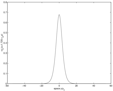
FIG. 1.: Fig.1 Variation of the form of the soliton $\varphi_{s}(y)$ with the velocity, $u$.

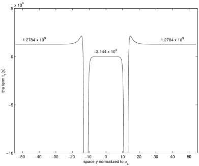
FIG. 2.: Fig.2 The function $t_{1}\left(y\right)$ for a particular soliton velocity, $u=1.725\,v_{d}$.

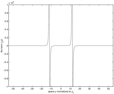
FIG. 3.: Fig.3 The function $t_{2}\left(y\right)$ of the Eq.(74) for the same $u$.

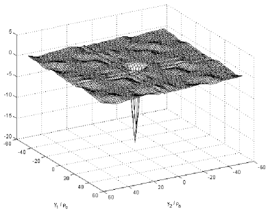
FIG. 4.: Fig.4 The perturbation to the correlation in physical space.

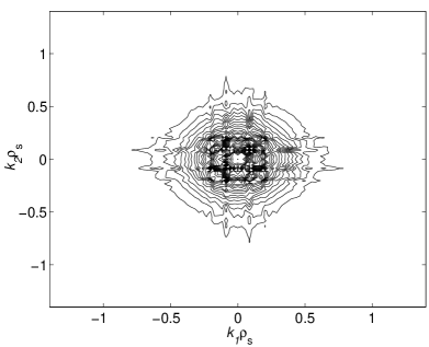
FIG. 5.: Fig.5 Contour plot of the spectrum of the vortex perturbed by the turbulent drift waves.

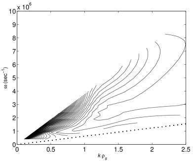
FIG. 6.: Fig.6 The contour plot of the frequency-wavenumber spectrum, with $\omega-ku=0$.

REFERENCES

- [1] F. Spineanu and M. Vlad, Phys. Rev. Letter 84, 4854 (2000)
- [2] D. Fyfe, D. Montgomery and G. Joyce, J. Plasma Phys. 17, 369 (1976).
- [3] D. Biskamp, Phys.Reports, 1997.
- [4] G.C. Craddock, P.H. Diamond and P.W. Terry, Phys. Fluids B 3, 304 (1991).
- [5] X.N. Su, W. Horton and P.J. Morrison, Phys. Fluids B 3, 921 (1991).
- [6] M. Kono and E. Miyashita, Phys. Fluids 31, 326 (1988).
- [7] T.Tajima, W.Horton,P.J.Morrison,S.Shutkeker, T. Kamimura, K.Mima and Y.Abe, Phys.Fluids B 3 938 (1991).
- [8] R.D. Hazeltine, D.D.Holm and P.J.Morrison, J.Plasma Phys.34 103 (1985).
- [9] J. Nycander, Phys.Fluids B 3 931 (1991).
- [10] R. Kinney, J.C. McWilliams and T. Tajima, Phys.Plasmas 2 3623 (1995).
- [11] F. Spineanu and M. Vlad, Comments Plasma Phys. 18, 115 (1997).
- [12] F. Spineanu, M.Vlad, J.-D. Reuss and J.H. Misguich, Plasma Physics Control. Fusion 41 (1999) 485.
- [13] J.D. Meiss and W. Horton, Phys. Fluids 25, 1838 (1982).
- [14] J.D. Meiss and W. Horton, Phys.Fluids 26 990 (1983).
- [15] P.J. Holmes, J.L.Lumley, Gal Berkooz, J. C. Mattingly and R.W. Wittenberg, Phys.Reports 287 337 (1997).
- [16] W. Horton, Phys.Reports 192 1 (1990).
- [17] J. A. Krommes, in Handbook of Plasma Physics edited by A. A. Galeev and R. N. Sydan (North-Holland, Amsterdam, 1984), Vol. 2, Chap. 5.5, p. 183.
- [18] J.H. Misguich and R.Balescu, Plasma Phys. 24, 284 (1982).
- [19] W. Y. Zhang and R. Balescu, Plasma Phys. Control. Fusion 29, 993 (1987); Plasma Phys. Control. Fusion 29, 1019 (1987).
- [20] P. W. Terry and P.H. Diamond, Phys. Fluids 28, 1419 (1985).
- [21] W. Horton, J. Liu, J.D.Meiss and J.E. Sedlak, Phys.Fluids 29, 1004, (1986).
- [22] P. C. Martin, E. D. Siggia and H. A. Rose, Phys. Rev. A 8, 423 (1973).
- [23] R. V. Jensen, J. Stat. Phys. 25, 183 (1981).
- [24] D. J. Amit, Field Theory, the Renormalization Group and Critical Phenomena, Singapore: World Scientific, (1984).
- [25] J. A. Krommes, Phys. Rev. E 53, 4865 (1996).
- [26] B.-G. Hong, Duk-In Choi and W. Horton, Jr., Phys. Fluids 29, 1872 (1986).
- [27] J.P. Boyd and B. Tan, Chaos, Solitons & Fractals 9, 2007 (1998).
- [28] I. S. Gradshtein and I. M. Ryzhik, Table of Integrals, series and products, Academic Press, 1980, formulas 8.322 and 1.431.1.
- [29] V. I. Karpman, Physica Scripta 20, 462, (1979).
- [30] G. Eilenberger, Solitons, (Mathematical methods for physicists). Springer Series in Solid-State Sciences, Vol. 19, Springer, Berlin, Heidelberg, 1981.
- [31] P.G. Drazin and R.S. Johnson, Solitons: an introduction, Cambridge Texts in Applied Mathematics, Cambridge University Press, Cambridge, 1989.
- [32] T. Schafer and E. V. Shuryak, Rev. Mod. Phys.70, 323 (1998).
- [33] F.Spineanu and M. Vlad, Physics of Plasmas, 4, 2106 (1997).
- [34] F.Spineanu, M. Vlad and J.H. Misguich, J.Plasma Phys. 51, 113 (1994).
- [35] F. Spineanu and M. Vlad, J.Plasma Phys. 54, 333 (1995).
- [36] T. Hwa and M. Kardar, Phys.Rev.A 45, 7002 (1992).