Elastic wave propagation along DNA.

Abstract

It is shown that information transmission inside a cell can occur by means of mechanical waves transmitted through DNA. The propagation of the waves is strongly dependent on the shape of the DNA thus proteins that change the shape of DNA can alter signal transmission. The overall effect is a method of signal processing by DNA binding proteins that creates a ”cellular communications network”.

The propagation of small amplitude disturbances through DNA is treated according to the mechanical theory of elastic rods. According to the theory four types of mechanical waves affecting extension(compression), twist, bend or shear can propagate through DNA. Each type of wave has unique characteristic properties. Disturbances affecting all wave types can propagate independently of each other. Using a linear approximation to the theory of motion of elastic rods, the dispersion of these waves is investigated. The phase velocities of the waves lies in the range $5\sim 8\r{A}/ps$ using constants suitable for a description of DNA. The dispersion of all wave types of arbitrary wave length is investigated for a straight, twisted rod.

Based on these findings, we propose all-atom numerical simulations of DNA to investigate the propagation of these waves as an alternative measure of the wave velocity and dispersion analysis.

Introduction

Our treatment of DNA is based on the hypothesis that such a well organized system as a cell must have a highly sophisticated system of communications. For instance, the cell cycle is the result of a series of complex self organized processes that must be well orchestrated. A model has been developed to demonstrate how these events may be initiated by critical concentrations of specific proteins which shift equilibrium to favor the advance of the cell cycle[1]. However, it is also known that the cell-cycle can be disrupted if conditions are not suitable. Similar arguments apply to virtually all cellular processes and in order to achieve the required checks and balances a method of communication is necessary.

Is there the possibility that information is transmitted through DNA electromagnetically instead of mechanically? In such case DNA will function as a transmission line which requires total internal reflection (TIR) of the radiation within the DNA. To achieve TIR, the wavelength of the radiation must be 5-10 times less than the diameter of the transmission line. Since the diameter of the DNA is close to 20 $\r{A}$ the radiation must have a wavelength close to 2 $\r{A}$. This wavelength is close to atomic dimensions so diffraction should dominate. Furthermore, the energy associated with this wavelength radiation is on the order of $10^{5}\ kcal/mol$ which is sufficient to destroy chemical bonds and therefore not easily managed biologically. For these reasons, we believe that the communication will be achieved mechanically.

The remainder of the paper will demonstrate that the mechanical properties of DNA have the necessary time and spatial dimension to support the propagation of information while interactions between proteins and DNA provide a mechanism by which this information is processed.

This manuscript is based on a continuous medium model of DNA. Such an approach is well known and widely used to describe solids, liquids and gases (see, for example [2, 3]). Thus, when we speak of infinitely small elements of volume, we shall always mean those which are ”physically” infinitely small, i.e. very small compared with wavelength or radius of curvature under consideration, but large compared with the distance between the atoms in DNA.

1 System of equation for the elastic rod dynamics

We utilize an elastic rod model described by [4] that has been parameterized to represent DNA [5]. The equations of motion are as follows:

$$\rho\left({\partial\vec{\gamma}\over\partial t}+\vec{\omega}\times\vec{\gamma}\right) = \hat{C}\cdot{\partial(\vec{\Gamma}-\vec{\Gamma}_{0}(s))\over\partial s}+\vec{\Omega}\times\left(\hat{C}\cdot\left(\vec{\Gamma}-\vec{\Gamma}_{0}\right)\right)$$ (1)

$$\hat{I}\cdot{\partial\vec{\omega}\over\partial t}+\vec{\omega}\times\left(\hat{I}\cdot\vec{\omega}\right) = \hat{D}\cdot{\partial(\vec{\Omega}-\vec{\Omega}_{0}(s))\over\partial s}+\vec{\Omega}\times\left(\hat{D}\cdot\left(\vec{\Omega}-\vec{\Omega}_{0}\right)\right)$$ (2)

$$+ \vec{\Gamma}\times\left(\hat{C}\cdot\left(\vec{\Gamma}-\vec{\Gamma}_{0}\right)\right)$$

$${\partial\vec{\Gamma}\over\partial t}+\vec{\omega}\times\vec{\Gamma} = {\partial\vec{\gamma}\over\partial s}+\vec{\Omega}\times\vec{\gamma}$$ (3)

$${\partial\vec{\Omega}\over\partial t}+\vec{\omega}\times\vec{\Omega} = {\partial\vec{\omega}\over\partial s}$$ (4)

In this system of equations, equation (1) represents the balance of force and linear momentum and equation (2) represents the balance of torque and angular momentum according to Newton’s Laws. Equations (3) and (4) are continuity relations expressed in a non-inertial reference frame. Here, $s$ and $t$ are independent variables representing time and fiducial arclength, respectively . The functions that we wish to study are the four three-vector functions $\vec{\Omega}$, $\vec{\Gamma}$, $\vec{\omega}$, and $\vec{\gamma}$.

The matrices $\hat{I}$, $\hat{C}$ and $\hat{D}$ and the scalar $\rho$ are as follows: Matrix $\hat{I}$ is the linear density of the moment of inertia tensor. Matrices $\hat{C}$ and $\hat{D}$ represent the elastic properties of the rod ($C_{3}$: Young’s modulus, $C_{1}$ and $C_{2}$: shear modulus, $D_{3}$: torsional rigidity, $D_{1}$ and $D_{2}$: bend stiffness). $\rho$ is the linear mass density and is equal to $3.22\times 10^{-15}\mbox{K/M}$ for an isotropic model of DNA. The matrices have the following values for an isotropic model of DNA:

$$I_{ik} = \left(\matrix{I&0&0\cr 0&I&0\cr 0&0&2I\cr}\right)\equiv\left(\matrix{4.03&0&0\cr 0&4.03&0\cr 0&0&8.06\cr}\right)\times 10^{-34}\left[KM\right]$$ (5)

$$C_{ik} = \left(\matrix{C_{1}&0&0\cr 0&C_{2}&0\cr 0&0&C_{3}\cr}\right)\equiv\left(\matrix{8.16&0&0\cr 0&8.16&0\cr 0&0&21.6\cr}\right)\times 10^{-10}\left[\frac{KM}{S^{2}}\right]$$ (6)

$$D_{ik} = \left(\matrix{D_{1}&0&0\cr 0&D_{2}&0\cr 0&0&D_{3}\cr}\right)\equiv\left(\matrix{2.7&0&0\cr 0&2.7&0\cr 0&0&2.06\cr}\right)\times 10^{-28}\left[\frac{KM^{3}}{S^{2}}\right]$$ (7)

For isotropic bending $C_{1}=C_{2}$ and shear $D_{1}=D_{2}$ we will denote $C=C_{1}=C_{2}$ and $D=D_{1}=D_{2}$. These definitions will be used below. The above values have been adapted from [6], [7].

In biological terminology the components of $\vec{\Gamma}$ correspond to the three DNA helical parameters describing translation $\vec{\Gamma}=(\mbox{shift,slide,rise})$ and the components of $\vec{\Omega}$ correspond to the three DNA helical parameters describing rotation $\vec{\Omega}=(\mbox{tilt,roll,twist})$. If we attach a local coordinate frame, denoted by $\{\vec{d}_{1},\vec{d}_{2},\vec{d}_{3}\}$, to each base-pair the axes will point in the direction of the major groove, minor groove and along the DNA helical axis, respectively. The shape of the DNA can be described by a three-dimensional vector function $\vec{r}(s,t)$ which is related to $\vec{\Gamma}$ and $\vec{\Omega}$ by a suitable mathematical integration.

In elastic rod terminology the three-dimensional vector function $\vec{r}(s,t)$ gives the centerline curve of the rod as a function of $s$ and $t$, showing only how the rod bends. To show the twist, shear and extension of the rod we must attach ”director” frames made of the orthogonal triples $\{\vec{d}_{1},\vec{d}_{2},\vec{d}_{3}\}$ at regular intervals along the rod. The director frames are evenly spaced along the rod when the rod is not extended and are all parallel to each other (with $\vec{d}_{3}$ pointing along the rod) when the rod is not bent or twisted. Any deformation of the rod will be indicated by a corresponding change in the orientation of the director frames.

The vector $\vec{\gamma}$ ($\vec{\Gamma}$) is the translational velocity of $\vec{r}$ in time (space):

$$\vec{\gamma}={\partial\vec{r}\over\partial t}\qquad\vec{\Gamma}={\partial\vec{r}\over\partial s}$$

The directors are of constant unit length, so the velocity of each director $\vec{\omega}$ ($\vec{\Omega}$) is always perpendicular to itself, and it must also be perpendicular to the axis of rotation of the local frame.

$${\partial\vec{d}_{k}\over\partial t}=\vec{\omega}\times\vec{d}_{k}\qquad{\partial\vec{d}_{k}\over\partial s}=\vec{\Omega}\times\vec{d}_{k}$$

We will denote $\vec{\Gamma}$ of the unstrained state by $\vec{\Gamma}_{0}$. In general an unstrained rod can have any shape. The most simple case is when the rod is straight with unit extension, $\vec{\Gamma}_{0}=\{0,0,1\}$, because in the unstrained state:

$${\partial\vec{r}_{3}\over\partial s}=\{0,0,1\}$$

Similarly, an unstressed elastic rod may have an intrinsic bend and/or twist, denoted by $\vec{\Omega}_{0}$, which must be subtracted from the total $\vec{\Omega}$ to give the dynamically active part. The simplest case is a rod with no intrinsic bend or twist $\vec{\Omega}=\{0,0,0\}$ and $\vec{\Gamma}_{0}=\{0,0,1\}$.

For short wave lengths (Section 2) we will suppose that $\vec{\Omega}_{0}=$ $(\Omega_{01},\Omega_{02},\Omega_{03})=const$ and $\vec{\Gamma}_{0}=(\Gamma_{01},\Gamma_{02},\Gamma_{03})=const$. In section 3 we will consider a straight rod with an intrinsic twist $\vec{\Omega}=\{0,0,\Omega_{0}\}$ and $\vec{\Gamma}=\{0,0,\Gamma_{0}\}$.

2 System for small amplitude waves

The results from this section are valid for any shape in which the curvature of the rod is much greater than the wavelength of the disturbance being propagated regardless of the intrinsic shape of the rod.

Let us search as usual for the equilibrium point of the system (1-4) by setting $\vec{\gamma}$, $\vec{\Gamma}$, $\vec{\omega}$ and $\vec{\Omega}$ to constants. It is easy to see that an equilibrium point of equations (1-4) is $\vec{\gamma}=\vec{\omega}=0$, $\vec{\Gamma}=\vec{\Gamma}_{0}$ and $\vec{\Omega}=\vec{\Omega}_{0}\;$

We shall suppose that each variable differs slightly from the equilibrium value so we retain only the linear terms in the equations. The linearized system (1-4) is:

$$\rho{\partial\vec{\gamma}\over\partial t} = \hat{C}\cdot{\partial\vec{\Gamma}\over\partial s}+\vec{\Omega}_{0}\times\left(\hat{C}\cdot\vec{\Gamma}\right)$$ (8)

$$\hat{I}\cdot{\partial\vec{\omega}\over\partial t} = \hat{D}\cdot{\partial\vec{\Omega}\over\partial s}+\vec{\Omega}_{0}\times\left(\hat{D}\cdot\vec{\Omega}\right)+\vec{\Gamma}_{0}\times\left(\hat{C}\cdot\vec{\Gamma}\right)$$ (9)

$${\partial\vec{\Gamma}\over\partial t} + \vec{\omega}\times\vec{\Gamma}_{0}={\partial\vec{\gamma}\over\partial s}+\vec{\Omega}_{0}\times\vec{\gamma}$$ (10)

$${\partial\vec{\Omega}\over\partial t} + \vec{\omega}\times\vec{\Omega}_{0}={\partial\vec{\omega}\over\partial s}$$ (11)

In the system (8-11) and further in this paper $\vec{\gamma}$, $\vec{\Gamma}$, $\vec{\omega}$ and $\vec{\Omega}$ denote the small deviations from the equilibrium values, e.g. $\vec{\Gamma}-\vec{\Gamma}_{0}\to\vec{\Gamma}$.

In the usual manner we search for a solution to (8-11) using harmonic analysis. We assume that each variable depends on time and space as follows:

$$\vec{G}_{i}(s,t)=\vec{G}_{i0}\cdot e^{\displaystyle{-i\omega t+iks}}$$ (12)

where $\vec{G}_{i}(s,t)$ denotes one of the four vector variables from the system of equations (8-11) and $\vec{G}_{i0}=const$ denotes its amplitude.

Let us substitute (12) to the system (8-11):

$$-i\omega\rho\vec{\gamma} = ik(\hat{C}\cdot\vec{\Gamma})+\vec{\Omega}_{0}\times\left(\hat{C}\cdot\vec{\Gamma}\right)$$ (13)

$$-i\omega(\hat{I}\cdot\vec{\omega}) = ik\left(\hat{D}\cdot\vec{\Omega}\right)+\vec{\Omega}_{0}\times\left(\hat{D}\cdot\vec{\Omega}\right)+\vec{\Gamma}_{0}\times\left(\hat{C}\cdot\vec{\Gamma}\right)$$ (14)

$$-i\omega\vec{\Gamma}+\vec{\omega}\times\vec{\Gamma}_{0} = ik\vec{\gamma}+\vec{\Omega}_{0}\times\vec{\gamma}$$ (15)

$$-i\omega\vec{\Omega}+\vec{\omega}\times\vec{\Omega}_{0} = ik\vec{\omega}$$ (16)

For short wavelength we search for solutions with $\omega\propto k$, so in the limit $k\to\infty$ we neglect all terms which contain cross products and the system (13-16) becomes:

$$(\omega^{2}\rho-k^{2}C)\vec{\Gamma}_{\bot} = 0$$ (17)

$$(\omega^{2}\rho-k^{2}C_{3})\Gamma_{3} = 0$$ (18)

$$(\omega^{2}I-k^{2}D)\vec{\Omega}_{\bot} = 0$$ (19)

$$(2\omega^{2}I-k^{2}D_{3})\Omega_{3} = 0$$ (20)

Here division into longitudinal and transversal components has been obtained by defining $\vec{\Gamma}_{\bot}\equiv(\Gamma_{1},\Gamma_{2},0)$ and $\vec{\Omega}_{\bot}\equiv(\Omega_{1},\Omega_{2},0)$.

Equations (17-20) represent four types of waves that can propagate in the elastic rod with velocity, $V$ (according to the order of equations above):

• Shear waves ($\vec{\Gamma}_{\bot}$):

  $$V_{Shear}=\sqrt{\frac{C}{\rho}}=\sqrt{8.16\cdot 10^{-10}[KM/s^{2}]\over 3.22\cdot 10^{-15}[K/M]}\approx 5.03\r{A}/ps$$ (21)

• Extension waves ($\Gamma_{3}$):

  $$V_{Extension}=\sqrt{\frac{C_{3}}{\rho}}=\sqrt{21.6\cdot 10^{-10}[KM/s^{2}]\over 3.22\cdot 10^{-15}[K/M]}\approx 8.2\r{A}/ps$$ (22)

• Bend waves ($\vec{\Omega}_{\bot}$):

  $$V_{Bend}=\sqrt{\frac{D}{I}}=\sqrt{2.7\cdot 10^{-28}[KM^{3}/s^{2}]\over 4.03\cdot 10^{-34}[KM]}\approx 8.2\r{A}/ps$$ (23)

• Twist waves ($\Omega_{3}$):

  $$V_{Twist}=\sqrt{\frac{D_{3}}{2I}}=\sqrt{2.06\cdot 10^{-28}[KM^{3}/s^{2}]\over 2\cdot 4.03\cdot 10^{-34}[KM]}\approx 5.0\r{A}/ps$$ (24)

These results were obtained for a rod with arbitrary shape because all terms that define the rod shape in equations (13-16) were omitted. So, if wavelength tends to zero (is the least space parameter of the problem) four wave types can propagate along the rod.

It is well known that the measurement of wave velocity is a usual method for determining elastic properties of solids. So, wave velocity (transversal and longitudinal) and Young’s modulus (shear modulus) are uniquely determined by formulae similar to the (21-24).

Hakim et al. [8] have determined the velocity of sound in DNA. Based on elastic constants obtained from [6], [7] and used in this work, the velocity is approximately two times less than that obtained by Hakim et al. [8].

Experiments to measure elastic properties of single DNA molecules have been reported using scanning tunnelling microscopy [9], fluorescence microscopy [10], fluorescence correlation spectroscopy [11], optical tweezers [12][13], bead techniques in magnetic fields [14] [15], optical microfibers [16], low energy electron point sources (electron holography) [17] and atomic force microscopy (AFM) [18]. Each method differs in the molecular properties probed, spatial and temporal resolution, molecular sensitivity and working environment, so each method gives close but not the same value of elastic constants. So if we evaluate extension/compression velocity using constants obtained from the data reported in [12] the result will be two times slower than the value reported here and based on data from [6] and [7].

3 Linear waves in the straight rod with no intrinsic bend or shear.

Here we concentrate our attention on the case of the straight, twisted rod with no intrinsic bend or shear. In this section we suppose that $\vec{\Omega}_{0}=(0,0,\Omega_{0})$ and $\vec{\Gamma}_{0}=(0,0,\Gamma_{0})$. As we will see this case allows for a complete analytical analysis of extension/compression (Section 3.1), twist (Section 3.2), and bend/shear (Section 3.3) waves of arbitrary wave length. Equations (8-11) in component form are:

$$\rho{\partial\gamma_{1}\over\partial t} = C\cdot{\partial\Gamma_{1}\over\partial s}-C\Omega_{0}\Gamma_{2}$$ (25)

$$\rho{\partial\gamma_{2}\over\partial t} = C\cdot{\partial\Gamma_{2}\over\partial s}+C\Omega_{0}\Gamma_{1}$$ (26)

$$\rho{\partial\gamma_{3}\over\partial t} = C_{3}\cdot{\partial\Gamma_{3}\over\partial s}$$ (27)

$$I\cdot{\partial\omega_{1}\over\partial t} = D\cdot{\partial\Omega_{1}\over\partial s}-D\Omega_{0}\Omega_{2}-C\Gamma_{0}\Gamma_{2}$$ (28)

$$I\cdot{\partial\omega_{2}\over\partial t} = D\cdot{\partial\Omega_{2}\over\partial s}+D\Omega_{0}\Omega_{1}+C\Gamma_{0}\Gamma_{1}$$ (29)

$$2I\cdot{\partial\omega_{3}\over\partial t} = D_{3}\cdot{\partial\Omega_{3}\over\partial s}$$ (30)

$${\partial\Gamma_{1}\over\partial t}+\Gamma_{0}\omega_{2} = {\partial\gamma_{1}\over\partial s}-\Omega_{0}\gamma_{2}$$ (31)

$${\partial\Gamma_{2}\over\partial t}-\Gamma_{0}\omega_{1} = {\partial\gamma_{2}\over\partial s}+\Omega_{0}\gamma_{1}$$ (32)

$${\partial\Gamma_{3}\over\partial t} = {\partial\gamma_{3}\over\partial s}$$ (33)

$${\partial\Omega_{1}\over\partial t}+\Omega_{0}\omega_{2} = {\partial\omega_{1}\over\partial s}$$ (34)

$${\partial\Omega_{2}\over\partial t}-\Omega_{0}\omega_{1} = {\partial\omega_{2}\over\partial s}$$ (35)

$${\partial\Omega_{3}\over\partial t} = {\partial\omega_{3}\over\partial s}$$ (36)

It is easy to see that equations (27) and (33) (also (30) and (36)) are independent from all other equations and describe extension (twist) waves. These two wave types will be discussed in the next two sections.

3.1 Sound (extension/compression) waves

From equations (27) and (33) it is easy to obtain two wave equations for the extension/compression waves:

$$\rho{\partial^{2}\gamma_{3}\over\partial t^{2}} - C_{3}{\partial^{2}\gamma_{3}\over\partial s^{2}}=0$$ (37)

$$\rho{\partial^{2}\Gamma_{3}\over\partial t^{2}} - C_{3}{\partial^{2}\Gamma_{3}\over\partial s^{2}}=0$$ (38)

These small amplitude waves have velocity (22) and these equations have an harmonic solution:

$$\Gamma_{3}=A_{1}\sin(s-t\sqrt{\frac{C_{3}}{\rho}})+A_{2}\cos(s-t\sqrt{\frac{C_{3}}{\rho}})$$ (41)

$$\gamma_{3}=B_{1}\sin(s-t\sqrt{\frac{C_{3}}{\rho}})+B_{2}\cos(s-t\sqrt{\frac{C_{3}}{\rho}})$$ (42)

where $A_{1,2}$ are arbitrary constants (wave amplitudes) and $B_{1,2}=\phantom{=}$ $-\sqrt{C_{3}/\rho}\;A_{1,2}$.

Using elastic constants obtained from data in [6] and [7] the velocity of sound in DNA is equal to $V_{sound}=8.2\r{A}/ps$ (see equation (22)) and dispersion is linear. This is the velocity of propagation of harmonic waves in DNA according to the linear approximation. In the linear approximation the amplitude of the wave must be small, but it can have any wavelength.

3.2 Twist waves

In the same manner equations (30) and (36) yield two wave equations which describe twist waves:

$$2I{\partial^{2}\omega_{3}\over\partial t^{2}} - D_{3}{\partial^{2}\omega_{3}\over\partial s^{2}}=0$$ (43)

$$2I{\partial^{2}\Omega_{3}\over\partial t^{2}} - D_{3}{\partial^{2}\Omega_{3}\over\partial s^{2}}=0$$ (44)

Linear solutions of these equations can be written as:

$$\Omega_{3}=P_{1}\sin(s-t\sqrt{\frac{D_{3}}{2I}})+P_{2}\cos(s-t\sqrt{\frac{D_{3}}{2I}})$$ (45)

$$\omega_{3}=Q_{1}\sin(s-t\sqrt{\frac{D_{3}}{2I}})+Q_{2}\cos(s-t\sqrt{\frac{D_{3}}{2I}})$$ (46)

where $P_{1,2}$ are the arbitrary constants (wave amplitudes) and $Q_{1,2}=\phantom{=}$ $-\sqrt{{D_{3}}/{2I}}\;P_{1,2}$.

These solutions describe twist waves with velocity $V_{twist}=\sqrt{\displaystyle{D_{3}}/{2I}}\approx 5.0\r{A}/ps$ (see equation (24)). In the general case, the solutions of these equations will be d’Alembertian waves described by (39-40). Again the dispersion law is linear.

3.3 Bend and Shear Waves

Substituting (12) into the remaining equations of system (25-36) yield:

$$-i\omega\rho\vec{\gamma}_{\bot} = ikC\vec{\Gamma}_{\bot}+C\left[\vec{\Omega}_{0}\times\vec{\Gamma}_{\bot}\right]$$ (47)

$$-i\omega I\vec{\omega}_{\bot} = ikD\vec{\Omega}_{\bot}+D\left[\vec{\Omega}_{0}\times\vec{\Omega}_{\bot}\right]+C\left[\vec{\Gamma}_{0}\times\vec{\Gamma}_{\bot}\right]$$ (48)

$$-i\omega\vec{\Gamma}_{\bot}+\left[\vec{\omega}_{\bot}\times\vec{\Gamma}_{0}\right] = ik\vec{\gamma}_{\bot}+\left[\vec{\Omega}_{0}\times\vec{\gamma}_{\bot}\right]$$ (49)

$$-i\omega\vec{\Omega}_{\bot}+\left[\vec{\omega}_{\bot}\times\vec{\Omega}_{0}\right] = ik\vec{\omega}_{\bot}$$ (50)

Here, the definitions $\vec{\gamma}_{\bot}\equiv(\gamma_{1},\gamma_{2},0)$, $\vec{\Gamma}_{\bot}\equiv(\Gamma_{1},\Gamma_{2},0)$, $\vec{\omega}_{\bot}\equiv(\omega_{1},\omega_{2},0)$ and $\vec{\Omega}_{\bot}\equiv(\Omega_{1},\Omega_{2},0)$ are used. This is an homogeneous system of linear equations with unknowns $\vec{\gamma}_{\bot}$, $\vec{\Gamma}_{\bot}$, $\vec{\omega}_{\bot}$ and $\vec{\Omega}_{\bot}$. Solutions other than the trivial solution exist only if the determinant of the coefficients is zero. This condition is satisfied if:

$$\left(\omega^{2}\rho-(k^{2}+\Omega_{0}^{2})C-{\rho\omega^{2}C\Gamma_{0}^{2}\left(\omega^{2}I-(k^{2}+\Omega_{0}^{2})D\right)\over\left(\omega^{2}I-(k^{2}+\Omega_{0}^{2})D\right)^{2}-4k^{2}D^{2}\Omega_{0}^{4}}\right)^{2}$$

$$=\left(2kC\Omega_{0}+{2k\rho D\omega^{2}C\Gamma_{0}\left(\vec{\Omega}_{0}\cdot\vec{\Gamma}_{0}\right)\over\left(\omega^{2}I-(k^{2}+\Omega_{0}^{2})D\right)^{2}-4k^{2}D^{2}\Omega_{0}^{4}}\right)^{2}$$ (51)

Let us discuss the untwisted rod ($\Omega_{0}=0$). Equation (51) yields:

$$\omega^{2}\rho-k^{2}C-{\rho\omega^{2}C\Gamma_{0}^{2}\over\omega^{2}I-k^{2}D}=0$$ (52)

It will be convenient to use dimensionless variables (marked by asterisk) $\omega^{*}=\omega\sqrt{I/C}$, $k^{*}=k\sqrt{I/\rho}$ in this section and define $G^{2}\equiv{D/I\over C/\rho}$. Equation (52) becomes(asterisks are omitted):

$$(\omega^{2}-k^{2})(\omega^{2}-G^{2}k^{2})=\Gamma_{0}^{2}\omega^{2},$$ (53)

with solutions:

$$\omega_{1,2,3,4}=\pm\frac{1}{2}\left\{\sqrt{[G+1]^{2}k^{2}+\Gamma^{2}_{0}}\pm\sqrt{[G-1]^{2}k^{2}+\Gamma^{2}_{0}}\right\}$$ (54)

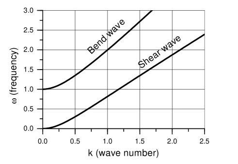
Figure 1: Dispersion of Bend/Shear Waves in DNA.

There are a total of four solutions. The $\pm$ sign before the braces merely changes the direction of propagation and will not be discussed further. The $\pm$ sign between the roots produces two different branches of solutions as presented in Fig.1. The ”upper” branch corresponds to bend waves and the ”lower” branch to shear waves.

For a rod of infinite length, any value of $\omega$ can be chosen that satisfies equation (53), but for a rod of finite length there will be an additional constraint that must be satisfied. If the rod is fixed at both ends then the usual restriction of having a node at each end applies. This introduces the constraint $L=(n/2)\lambda$ between the length of the rod, $L$, and the possible wavelengths, $\lambda$, so that only discrete points along either sub-branch in Figure 1 will be observed.

4 Conclusion.

The primary results are that, in the linear approximation, four different types of waves can propagate through a uniform elastic rod. These waves correspond to extension(compression), twist, bend and shear. An extension or twist wave will propagate without exciting other modes or changing shape, and it has a linear dispersion relation. Bend and shear waves behave rather differently and have a nonlinear dispersion relation. Each type obeys a dispersion law that describes two additional sub-branches.

Utilizing constants suitable for DNA we find that, in the limit of small wavelengths, extension and bend propagate with a velocity of approximately 8Å/ps and twist and shear propagate with a velocity of approximately 5Å/ps.

Is is also significant that the dispersion relation for bend and shear waves is coupled with the inherent twist of DNA. We propose that these physical phenomena enable proteins interacting with DNA to accomplish highly sophisticated tasks. For example the difference in extension and twist velocities can be utilized to measure the distance between two points on the DNA. Since the dispersion law for bend and shear waves depends on intrinsic twist, a mechanism for measuring DNA topology exists because of the relation between twist, linking number and writhe. Other protein-protein communications can certainly be established to assist cellular mechanisms.

4.1 Suggestion for a simulation experiment

We suggest a molecular dynamics simulation experiment to check the correspondence between the linear theory of the propagation of waves in elastic rods and an all atom simulation of DNA. In all-atom molecular dynamics simulations of DNA the number of base pairs that can be simulated for a significant length of time is from tens to less than hundreds of base pairs. For a simulation of DNA with fixed ends it is sufficient to apply a sharp impulse ($\delta$ function excitation) to one end of the DNA and measure the time of propagation of this disturbance to the other end as a measure of the velocity of extension/compression waves in DNA according to equation (22). The propagation of twist can be similarly tested by applying a torque.

To measure dispersion one must make some simple calculations before the simulation and then excite one end of the DNA with a driving force of the appropriate frequency. In this manner a standing wave can be established in the DNA. The wave frequency and wave number ($2\pi/\lambda$) are related by the well known relation:

$$\omega=V_{Wave}k$$ (55)

where $\omega=2\pi f$ is the wave frequency, $V_{Wave}$ is the wave velocity and $k=2\pi/\lambda$ is the wavelength. In this case the wave length (wave number) is easy to evaluate:

$$L=n{\lambda\over 2},\qquad\mbox{where n=1,2,3,.. }$$ (56)

and $f$ is the frequency of the driving oscillation. The values obtained from simulation can be compared with the number obtained from formula (53 or 53) as a means of correcting our choice of constants.

5 Acknowledgement

We express our thanks to Dr. Jan-Ake Gustafsson, Dr. Iosif Vaisman and Dr. Yaoming Shi for stimulating and helpful discussions. We would also like to thank Yaoming Shi for a critical reading of the manuscript.

This work was conducted in the Theoretical Molecular Biology Laboratory which was established under NSF Cooperative Agreement Number OSR-9550481/LEQSF (1996-1998)-SI-JFAP-04 and supported by the Office of Naval Research (NO-0014-99-1-0763).

References

- [1] John J. Tyson, Bela Novak, Garrett M. Odell, Kathy Chen and Dennis Thron. Chemical kinetic theory: understanding the cell-cycle regulation. Trends Biochem. Sci. 21, 89-96, (1996).
- [2] Landau L.D., Lifshitz E.M. Fluid Mechanics. Pergamon Press. 1959.
- [3] Landau L.D., Lifshitz E.M. Electrodynamics of Continous Media. Pergamon Press. 1960.
- [4] J.C.Simo, J.E.Marsden, P.S.Krishnaprasad, Archive for Rational Mechanics and Analysis, 104, 125-184,(1988).
- [5] a) Yaoming Shi, Andrey E. Borovik, and John E. Hearst. Elastic rod model incorporating shear extension, generalized nonlinear Schrödinger equations, and novel closed-form solutions for supercoiled DNA. J. Chem. Phys. 103,(8),3166-3183, (1995). b) Martin McClain, Yaoming Shi, T.C.Bishop, J.E.Hearst. Visualization of Exact Hamiltonian Dynamics Solutions. (to be published).
- [6] J.D.Moroz, P.Nelson, Entropic elasticity of twist-storing polymers, Macromolecules, 31, 6333-6347, (1998).
- [7] C. Bouchiat, M. Mzard. Elasticity model of a supercoiled DNA molecule, Phys. Rev. Lett. 80,(7),1556-1559, (1998).
- [8] M.B.Hakim, S.M.Lindsay, J.Powell. The Speed of Sound in DNA. Biopolymers, 23, 1185-1192 (1984)
- [9] Guckenberger R., Heim M., Cevc G., Knapp H.F., Wiegrbe W., Hillebrand A. Science 266, 1994, 1538-1540.
- [10] Yanagida M., Hiraoka Y., Katsura I., Cold Spring Harbor Symp. Quant. Biol. 47, 1983, 177.
- [11] Wennmalm S., Edman L., Rigler R. Proc. Natl. Acad. Sci. 94, 1997, 10641-10646.
- [12] Smith S.B., Cui Y., Bustamante C. Science. 271, 1996, 759-799.
- [13] Wang D.W., Yin H., Landick R., Gelles J., Block S.M. Biophys. J. 71, 1997, 1335-1346.
- [14] Smith S.B., Finzi L., Bustamante C. Science. 258, 1992, 1122-1126.
- [15] Strick T.R., Allemand J.F., Bensimon D., Bensimon A., Croquette V. Science. 271, 1996, 1835-1837.
- [16] Ph., Lebrun A., Heller Ch., Lavery R., Viovy J., Chatenay D., Caron F. Science. 271, 1996, 792-794.
- [17] Fink H. W., Schnenberger Ch. Science. 398, 1999, 407-410.
- [18] Hansma H.G., Sinsheimer R.L., Li M.Q., Hansma P.K. Nucleic Acids Res. 20, 1991, 3585-3590.
- [19] Bishop T., Zhmudsky O. Currents in Computational Molecular Biology 2001. Les Publications CRM, Montreal, 2001. Information Transmission along DNA. p. 105-106. ISBN 2-921120-35-6.