Abstract

Physically speaking, the delta function like beam-beam nonlinear forces at interaction points (IPs) act as a sum of delta function nonlinear multipoles. By applying the general theory established in ref. [1], in this paper we investigate analytically the beam-beam interaction limited dynamic apertures and the corresponding beam lifetimes for both the round and the flat beams. Relations between the beam-beam limited beam lifetimes and the beam-beam tune shifts are established, which show clearly why experimentally one has always a maximum beam-beam tune shift, $\xi_{y,max}$, around 0.045 for e⁺e^- circular colliders, and why one can use round beams to double this value approximately. Comparisons with some machine parameters are given. Finally, we discuss the mechanism of the luminosity reduction due to a definite collision crossing angle.

Analytical Estimation of the Beam-Beam
Interaction Limited Dynamic Apertures
and Lifetimes in e⁺e^- Circular Colliders
J. Gao
Laboratoire de L’Accélérateur Linéaire,
IN2P3-CNRS et Université de Paris-Sud, BP 34, 91898 Orsay cedex, France

1 Introduction

Beam-beam interactions in circular colliders have many influences on the performance of the machines, and the most important effect is that beam-beam interactions contribute to the limitations on dynamic apertures and beam lifetimes. Due to the importance of this subject, enormous efforts have been made to calculate incoherent and coherent beam-beam forces, to simulate beam-beam effects, to find the difference between flat and round colliding beams, and to establish analytical formulae to estimate the maximum beam-beam tune shift [2]-[20]. Physically speaking, the delta function like beam-beam nonlinear forces at interaction points (IPs) act as a sum of delta function nonlinear multipoles. In ref. [1] we have established a general theory to study analytically in detail the delta function multipoles and their combined effects on the dynamic apertures in circular storage rings, and in this paper we will apply these general analytical formulae to the case of beam-beam interactions and find the corresponding beam dynamic apertures and beam lifetimes. We will show quantitatively why there exists a maximum beam-beam tune shift, $\xi_{y,max}$, around 0.045 for flat beams in e⁺e^- circular colliders, and why this number can be almost doubled for round colliding beams. Applications to some machine parameters are also given. In this paper we will restrict ourselves to the discussion of e⁺e^- circular colliders since the treatment for the hadron colliders will be somewhat different and more difficult. Finally, we discuss beam-beam effects with a definite crossing angle.

2 Beam-beam interactions

For two head-on colliding bunches, the incoherent kick felt by each particle can be calculated as [13]:

$$\delta y^{\prime}+i\delta x^{\prime}=-{N_{e}r_{e}\over\gamma_{*}}f(x,y,\sigma_{x},\sigma_{y})$$ (1)

where $x^{\prime}$ and $y^{\prime}$ are the horizontal and vertical slopes, $N_{e}$ is the particle population in the bunch, $r_{e}$ is the electron classical radius (2.818$\times 10^{-15}$ m), $\sigma_{x}$ and $\sigma_{y}$ are the standard deviations of the transverse charge density distribution of the counter-rotating bunch at IP, $\gamma_{*}$ is the normalized particle’s energy, and $*$ denotes the test particle and the bunch to which the test particle belongs. When the bunch is Gaussian $f(x,y,\sigma_{x},\sigma_{y})$ can be expressed by Basseti-Erskine formula [10]:

$$f(x,y,\sigma_{x},\sigma_{y})=\sqrt{2\pi\over\sigma_{x}^{2}-\sigma_{y}^{2}}\times$$

$$\left(w\left({x+iy\over\sqrt{2(\sigma_{x}^{2}-\sigma_{y}^{2})}}\right)-\exp\left(-{x^{2}\over 2\sigma_{x}^{2}}-{y^{2}\over 2\sigma_{y}^{2}}\right)w\left({{\sigma_{y}\over\sigma_{x}}x+i{\sigma_{x}\over\sigma_{y}}y\over\sqrt{2(\sigma_{x}^{2}-\sigma_{y}^{2})}}\right)\right)$$ (2)

where $w$ is the complex error function expressed as

$$w(z)=\exp(-z^{2})(1-{\rm erf}(-iz))$$ (3)

For the round beam (RB) and the flat beam (FB) cases one has the incoherent beam-beam kicks expressed as [4][12][13]:

$$\delta r^{\prime}=-{2N_{e}r_{e}\over\gamma_{*}r}\left(1-\exp\left(-{r^{2}\over 2\sigma^{2}}\right)\right)\qquad({\rm RB},\sigma_{x}=\sigma_{y}=\sigma)$$ (4)

$$\delta x^{\prime}=-{2\sqrt{2}N_{e}r_{e}\over\gamma_{*}\sigma_{x}}\exp\left(-{x^{2}\over 2\sigma_{x}^{2}}\right)\int_{0}^{x\over\sqrt{2}\sigma_{x}}\exp(u^{2})du\qquad({\rm FB},\sigma_{x}>>\sigma_{y})$$ (5)

$$\delta y^{\prime}=-{\sqrt{2\pi}N_{e}r_{e}\over\gamma_{*}\sigma_{x}}\exp\left(-{x^{2}\over 2\sigma_{x}^{2}}\right){\rm erf}\left({y\over\sqrt{2}\sigma_{y}}\right)\qquad({\rm FB},\sigma_{x}>>\sigma_{y})$$ (6)

where $r=\sqrt{x^{2}+y^{2}}$. Now we want to calculate the average kick felt by the test particle since the probability to find the transverse displacement of the test particle is not constant (in fact, the probability function is the same as the charge distribution of the bunch to which the test particle belongs in lepton machines due to synchrotron radiations). In the following we assume that the transverse sizes for the two colliding bunches at IP are exactly the same. For the round beam case after averaging one gets[4][14]:

$$\delta\bar{r}^{\prime}=-{2N_{e}r_{e}\over\gamma_{*}\bar{r}}\left(1-\exp\left(-{\bar{r}^{2}\over 4\sigma^{2}}\right)\right)\qquad({\rm RB})$$ (7)

Although this expression is the same as that of the coherent beam-beam kick for round beams, one should keep in mind that we are not finding coherent beam-beam kick originally, and the difference will be obvious when we treat the vertical motion in the case of flat beams. For the flat beam case, we will treat the horizontal and vertical planes separately. As far as the horizontal kick is concerned, the horizontal kick depends only on one displacement variable just similar to the round beam case, we will use its coherent form expressed as follows [12][14]:

$$\delta x^{\prime}=-{2N_{e}r_{e}\over\gamma_{*}\sigma_{x}}\exp\left(-{x^{2}\over 4\sigma_{x}^{2}}\right)\int_{0}^{x\over 2\sigma_{x}}\exp(u^{2})du\qquad({\rm FB})$$ (8)

where $\sigma_{x}$ in the incoherent formula in ref. [12] has been replaced by $\Sigma_{x}=\sqrt{2}\sigma_{x}$ (for two identical Gaussian colliding beams) according to Hirata theorem demonstrated in the appendix A of ref. [14]. As for the vertical kick, however, one has to make an average over eq. 6 with the horizontal probability distribution function of the test particle, and one gets [13]:

$$\delta y^{\prime}=-{\sqrt{2\pi}N_{e}r_{e}\over\gamma_{*}\sigma_{x}}<\exp\left(-{x^{2}\over 2\sigma_{x}^{2}}\right)>_{x}{\rm erf}\left({y\over\sqrt{2}\sigma_{y}}\right)\qquad({\rm FB})$$ (9)

where $<>_{x}$ means the average over the horizontal probability distribution function of the test particle, and for two identical colliding Gaussian beams $<>_{x}=1/\sqrt{2}$. It is obvious that eq. 9 is not the expression for the coherent beam-beam kick. The average over eqs. 4 and 6 is only a technical operation to simplify (or to make equivalence) a two dimensional problem to a one dimensional one. To study both round and flat beam cases, we expand $\delta\bar{r}^{\prime}$ at $x=0$ (for round beam we study only vertical plane since the formalism in the horizontal plane is the same), $\delta x^{\prime}$ and $\delta y^{\prime}$ expressed in eqs. 7, 8 and 9, respectively, into Taylor series:

$$\delta_{y}^{\prime}={N_{e}r_{e}\over\gamma_{*}}({1\over 2\sigma^{2}}y-{1\over 16\sigma^{4}}y^{3}+{1\over 192\sigma^{6}}y^{5}-{1\over 3072\sigma^{8}}y^{7}$$

$$+{1\over 61440\sigma^{10}}y^{9}-{1\over 1474560\sigma^{12}}y^{11}+{1\over 41287680\sigma^{14}}y^{13}-\cdot\cdot\cdot)\qquad({\rm RB})$$ (10)

$$\delta_{x}^{\prime}=-{N_{e}r_{e}\over 2\gamma_{*}}({2\over\sigma_{x}^{2}}x-{1\over 3\sigma_{x}^{4}}x^{3}+{1\over 30\sigma_{x}^{6}}x^{5}-{1\over 420\sigma_{x}^{8}}x^{7}$$

$$+{1\over 7560\sigma_{x}^{10}}y^{9}-{1\over 166320\sigma_{x}^{12}}x^{11}+{1\over 4324320\sigma_{x}^{14}}x^{13}-\cdot\cdot\cdot)\qquad({\rm FB})$$ (11)

$$\delta_{y}^{\prime}=-{N_{e}r_{e}\over\sqrt{2}\gamma_{*}}({2\over\sigma_{x}\sigma_{y}}y-{1\over 3\sigma_{x}\sigma_{y}^{3}}y^{3}+{1\over 20\sigma_{x}\sigma_{y}^{5}}y^{5}-{1\over 168\sigma_{x}\sigma_{y}^{7}}y^{7}$$

$$+{1\over 1728\sigma_{x}\sigma_{y}^{9}}y^{9}-{1\over 21120\sigma_{x}\sigma_{y}^{11}}y^{11}+{1\over 299520\sigma_{x}\sigma_{y}^{13}}y^{13}-\cdot\cdot\cdot)\qquad({\rm FB})$$ (12)

The differential equations of the motion of the test particle in the transverse planes can be expressed as:

$${d^{2}y\over ds^{2}}+K_{y}(s)y=-{N_{e}r_{e}\over\gamma_{*}}({1\over 2\sigma^{2}}y-{1\over 16\sigma^{4}}y^{3}+{1\over 192\sigma^{6}}y^{5}$$

$$-{1\over 3072\sigma^{8}}y^{7}+{1\over 61440\sigma^{10}}y^{9}-{1\over 1474560\sigma^{12}}y^{11}$$

$$+{1\over 41287680\sigma^{14}}y^{13}-\cdot\cdot\cdot)\sum_{k=-\infty}^{\infty}\delta(s-kL)\qquad({\rm RB})$$ (13)

$${d^{2}x\over ds^{2}}+K_{x}(s)x=-{N_{e}r_{e}\over 2\gamma_{*}}({2\over\sigma_{x}^{2}}x-{1\over 3\sigma_{x}^{4}}x^{3}+{1\over 30\sigma_{x}^{6}}x^{5}$$

$$-{1\over 420\sigma_{x}8}x^{7}+{1\over 7560\sigma_{x}^{10}}x^{9}-{1\over 166320\sigma_{x}^{12}}x^{11}$$

$$+{1\over 4324320\sigma_{x}^{14}}x^{13}-\cdot\cdot\cdot)\sum_{k=-\infty}^{\infty}\delta(s-kL)\qquad({\rm FB})$$ (14)

$${d^{2}y\over ds^{2}}+K_{y}(s)y=-{N_{e}r_{e}\over\sqrt{2}\gamma_{*}}({2\over\sigma_{x}\sigma_{y}}y-{1\over 3\sigma_{x}\sigma_{y}^{3}}y^{3}+{1\over 20\sigma_{x}\sigma_{y}^{5}}y^{5}$$

$$-{1\over 168\sigma_{x}\sigma_{y}^{7}}y^{7}+{1\over 1728\sigma_{x}\sigma_{y}^{9}}y^{9}-{1\over 21120\sigma_{x}\sigma_{y}^{11}}y^{11}$$

$$+{1\over 299520\sigma_{x}\sigma_{y}^{13}}y^{13}-\cdot\cdot\cdot)\sum_{k=-\infty}^{\infty}\delta(s-kL)\qquad({\rm FB})$$ (15)

where $K_{x}(s)$ and $K_{y}(s)$ describe the linear focusing of the lattice in the horizontal and vertical planes. The corresponding Hamiltonians are expressed as:

$$H={p_{y}^{2}\over 2}+{K_{y}(s)\over 2}y^{2}+{N_{e}r_{e}\over\gamma_{*}}({1\over 4\sigma^{2}}y^{2}-{1\over 64\sigma^{4}}y^{4}+{1\over 1152\sigma^{6}}y^{6}$$

$$-{1\over 24576\sigma^{8}}y^{8}+\cdot\cdot\cdot)\sum_{k=-\infty}^{\infty}\delta(s-kL)\qquad({\rm RB})$$ (16)

$$H_{x}={p_{x}^{2}\over 2}+{K_{x}(s)\over 2}x^{2}+{N_{e}r_{e}\over 2\gamma_{*}}({1\over\sigma_{x}^{2}}x^{2}-{1\over 12\sigma_{x}^{4}}x^{4}+{1\over 180\sigma_{x}^{6}}x^{6}$$

$$-{1\over 3360\sigma_{x}^{8}}x^{8}+\cdot\cdot\cdot)\sum_{k=-\infty}^{\infty}\delta(s-kL)\qquad({\rm FB})$$ (17)

$$H_{y}={p_{y}^{2}\over 2}+{K_{y}(s)\over 2}y^{2}+{N_{e}r_{e}\over\sqrt{2}\gamma_{*}}({1\over\sigma_{x}\sigma_{y}}y^{2}-{1\over 12\sigma_{x}\sigma_{y}^{3}}y^{4}+{1\over 120\sigma_{x}\sigma_{y}^{5}}y^{6}$$

$$-{1\over 1344\sigma_{x}\sigma_{y}^{7}}y^{8}+\cdot\cdot\cdot)\sum_{k=-\infty}^{\infty}\delta(s-kL)\qquad({\rm FB})$$ (18)

where $p_{x}=dx/ds$ and $p_{y}=dy/ds$.

3 Review of the general analytical formulae for dynamic apertures

In ref. [1] we have studied analytically the one dimensional ($y=0$) dynamic aperture of a storage ring described by the following Hamiltonian:

$$H={p^{2}\over 2}+{K(s)\over 2}x^{2}+{1\over 3!B\rho}{\partial^{2}B_{z}\over\partial x^{2}}x^{3}L\sum_{k=-\infty}^{\infty}\delta(s-kL)$$

$$+{1\over 4!B\rho}{\partial^{3}B_{z}\over\partial x^{3}}x^{4}L\sum_{k=-\infty}^{\infty}\delta(s-kL)+\cdot\cdot\cdot$$ (19)

where

$$B_{z}=B_{0}(1+xb_{1}+x^{2}b_{2}+x^{3}b_{3}+x^{4}b_{4}+\cdot\cdot\cdot+x^{m-1}b_{m-1}+\cdot\cdot\cdot)$$ (20)

The dynamic aperture corresponding to each multipole is given as:

$$A_{dyna,2m,x}(s)=\sqrt{2\beta_{x}(s)}\left({1\over m\beta_{x}^{m}(s_{2m})}\right)^{1\over 2(m-2)}\left({\rho\over|b_{m-1}|L}\right)^{1/(m-2)}$$ (21)

where $s_{2m}$ is the location of the $2m$th multipole, $\beta_{x}(s)$ is the beta function in $x$ plane. Since these results are general, we have tried to avoid assigning the freedom of motion, $x$, a specific name, such as horizontal, or vertical plane.

4 Beam-beam limited dynamic apertures

To make use of the general dynamic aperture formulae recalled in section 3, one needs only to find the equivalence relations by comparing three Hamiltonians expressed in eqs. 16, 17, and 18 with eq. 19, and it is found by analogy that:

$${b_{m-1}\over\rho}L={N_{e}r_{e}\over C_{m,RB}\gamma_{*}\sigma^{m}}\qquad({\rm RB})$$ (22)

$${b_{m-1}\over\rho}L={N_{e}r_{e}\over C_{m,FB,x}2\gamma_{*}\sigma_{x}^{m}}\qquad({\rm FB},x)$$ (23)

$${b_{m-1}\over\rho}L={N_{e}r_{e}\over C_{m,FB,y}\sqrt{2}\gamma_{*}\sigma_{x}\sigma_{y}^{m-1}}\qquad({\rm FB},y)$$ (24)

where $C_{m,RB}$, $C_{m,FB,x}$, and $C_{m,FB,y}$ are given in Table 1.

m	4	6	8	10	12	14
$C_{m,RB}$	16	192	3072	61440	1474560	41287680
$C_{m,FB,x}$	3	30	420	7560	166320	4324320
$C_{m,FB,y}$	3	20	168	1728	21120	299520

Table 1: summary of multipole coefficients

Now by inserting eqs. 22-24 into eq. 21 one can calculate dynamic apertures of different multipoles due to nonlinear beam-beam forces. For example, one can get the dynamic apertures due to the beam-beam octupole nonlinear force:

$$A_{dyna,8,y}(s)={\sqrt{\beta_{y}(s)}\over\beta_{y}(s_{IP})}\sqrt{\rho\over|b_{3}|L}$$

$$={\sqrt{\beta_{y}(s)}\over\beta_{y}(s_{IP})}\left({16\gamma_{*}\sigma^{4}\over N_{e}r_{e}}\right)^{1/2}\qquad({\rm RB})$$ (25)

$$A_{dyna,8,x}(s)={\sqrt{\beta_{x}(s)}\over\beta_{x}(s_{IP})}\sqrt{\rho\over|b_{3}|L}$$

$$={\sqrt{\beta_{x}(s)}\over\beta_{x}(s_{IP})}\left({6\gamma_{*}\sigma_{x}^{4}\over N_{e}r_{e}}\right)^{1/2}\qquad({\rm FB})$$ (26)

$$A_{dyna,8,y}(s)={\sqrt{\beta_{y}(s)}\over\beta_{y}(s_{IP})}\sqrt{\rho\over|b_{3}|L}$$

$$={\sqrt{\beta_{y}(s)}\over\beta_{y}(s_{IP})}\left({3\sqrt{2}\gamma_{*}\sigma_{x}\sigma_{y}^{3}\over N_{e}r_{e}}\right)^{1/2}\qquad({\rm FB})$$ (27)

where $s_{IP}$ is the IP position. Given the dynamic aperture of the ring without the beam-beam effect as $A_{x,y}$, the total dynamic aperture including the beam-beam effect can be estimated usually as:

$$A_{total,x,y}(s)={1\over\sqrt{{1\over A_{x,y}(s)^{2}}+{1\over A_{bb,x,y}(s)^{2}}}}$$ (28)

In the following we will consider the case of $A_{total,x,y}(s)\approx A_{bb,x,y}(s)$. If we measure the beam-beam interaction limited dynamic apertures by the beam sizes (the normalized beam-beam limited dynamic aperture), one gets:

$${\cal R}_{y,8}={A_{dyna,8,y}(s)\over\sigma_{*}(s)}=\left({16\gamma_{*}\sigma^{2}\over N_{e}r_{e}\beta_{y}(s_{IP})}\right)^{1/2}\qquad({\rm RB})$$ (29)

$${\cal R}_{x,8}={A_{dyna,8,x}(s)\over\sigma_{*,x}(s)}=\left({6\gamma_{*}\sigma_{x}^{2}\over N_{e}r_{e}\beta_{x}(s_{IP})}\right)^{1/2}\qquad({\rm FB})$$ (30)

$${\cal R}_{y,8}={A_{dyna,8,y}(s)\over\sigma_{*,y}(s)}=\left({3\sqrt{2}\gamma_{*}\sigma_{x}\sigma_{y}\over N_{e}r_{e}\beta_{y}(s_{IP})}\right)^{1/2}\qquad({\rm FB})$$ (31)

Recalling and using the definitions of the beam-beam tune shifts $\xi_{x}$ and $\xi_{y}$ in eqs. 32 and 33:

$$\xi_{x}^{*}={N_{e}r_{e}\beta_{x,IP}\over 2\pi\gamma^{*}\sigma_{x}(\sigma_{x}+\sigma_{y})}$$ (32)

$$\xi_{y}^{*}={N_{e}r_{e}\beta_{y,IP}\over 2\pi\gamma^{*}\sigma_{y}(\sigma_{x}+\sigma_{y})}$$ (33)

one can simplify the above defined normalized dynamic apertures. As general results one finds:

$${\cal R}_{y,2m}={A_{dyna,2m,y}(s)\over\sigma_{*,y}(s)}=\left({2^{m-2\over 2}C_{m,RB}\over 4\pi\sqrt{m}\xi_{y}^{*}}\right)^{1\over m-2}\qquad({\rm RB})$$ (34)

$${\cal R}_{x,2m}={A_{dyna,2m,x}(s)\over\sigma_{*,x}(s)}=\left({2^{m-2\over 2}C_{m,FB,x}\over 2\sqrt{m}\pi\xi_{x}^{*}}\right)^{1\over m-2}\qquad({\rm FB})$$ (35)

$${\cal R}_{y,2m}={A_{dyna,2m,y}(s)\over\sigma_{*,y}(s)}=\left({2^{m-2\over 2}C_{m,FB,y}\over\sqrt{2m}\pi\xi_{y}^{*}}\right)^{1\over m-2}\qquad({\rm FB})$$ (36)

Obviously, the normalized beam-beam effect limited dynamic apertures are determined only by the beam-beam tune shifts. The impact of this discovery will be more appreciated later. When the higher order multipoles effects ($2m>8$) can be neglected eqs. 25, 26 and 27 give very good approximations dynamic apertures limited by one beam-beam IP. If there are $N_{IP}$ interaction points in a ring the dynamic apertures described in eqs. 25 and 27 will be reduced by a factor of $\sqrt{N_{IP}}$ (if these $N_{IP}$ interaction points can be regarded as independent).

5 Beam lifetime due to beam-beam
interactions

We take the beam-beam limited dynamic aperture as the rigid mechanical boundary, i.e., those particles which walk beyond this virtual boundary will be regarded lost instantaneously. Based on this physical point of view we can calculate the beam lifetime due to the nonlinear beam-beam effect:

$$\tau_{bb}=={\tau_{y}\over 2}\left({\sigma_{y}(s)^{2}\over A_{dyna,y}(s)^{2}}\right)\exp\left({A_{dyna,y}(s)^{2}\over\sigma_{y}(s)^{2}}\right)$$ (37)

where $\tau_{y}$ is the synchrotron radiation damping time in vertical plane. It is interesting to note that eq. 37 is similar to but different from the quantum lifetime forluma [21] where that $\sigma_{y}(s)^{2}$ is used instead of $2\sigma_{y}(s)^{2}$. The reason is that the quantum radiation results in energy fluctuations of an electron and $2\sigma_{y}(s)^{2}$ corresponds to the average of the square of the oscillation amplitude, however, the dynamic apertures calculated above due to nonlinear forces are relevant only to the projected motions. When the beam-beam octupole nonlinear force dominates the dynamic aperture, by inserting eqs. 29, 30, and 31 into eq. 37, or inserting eqs. 34, 35, and 36 into eq. 37 one gets:

$$\tau_{bb,y}^{*}={\tau_{y}^{*}\over 2}\left({16\gamma_{*}\sigma^{2}\over N_{e}r_{e}\beta_{y}(s_{IP})}\right)^{-1}\exp\left({16\gamma_{*}\sigma^{2}\over N_{e}r_{e}\beta_{y}(s_{IP})}\right)\qquad({\rm RB})$$ (38)

$$\tau_{bb,x}^{*}={\tau_{x}^{*}\over 2}\left({6\gamma_{*}\sigma_{x}^{2}\over N_{e}r_{e}\beta_{x}(s_{IP})}\right)^{-1}\exp\left({6\gamma_{*}\sigma_{x}^{2}\over N_{e}r_{e}\beta_{x}(s_{IP})}\right)\qquad({\rm FB})$$ (39)

$$\tau_{bb,y}^{*}={\tau_{y}^{*}\over 2}\left({3\sqrt{2}\gamma_{*}\sigma_{x}\sigma_{y}\over N_{e}r_{e}\beta_{y}(s_{IP})}\right)^{-1}\exp\left({3\sqrt{2}\gamma_{*}\sigma_{x}\sigma_{y}\over N_{e}r_{e}\beta_{y}(s_{IP})}\right)\qquad({\rm FB})$$ (40)

or

$$\tau_{bb,y}^{*}={\tau_{y}^{*}\over 2}\left({4\over\pi\xi_{y}^{*}}\right)^{-1}\exp\left({4\over\pi\xi_{y}^{*}}\right)\qquad({\rm RB})$$ (41)

$$\tau_{bb,x}^{*}={\tau_{x}^{*}\over 2}\left({3\over\pi\xi_{x}^{*}}\right)^{-1}\exp\left({3\over\pi\xi_{x}^{*}}\right)\qquad({\rm FB})$$ (42)

$$\tau_{bb,y}^{*}={\tau_{y}^{*}\over 2}\left({3\over\sqrt{2}\pi\xi_{y}^{*}}\right)^{-1}\exp\left({3\over\sqrt{2}\pi\xi_{y}^{*}}\right)\qquad({\rm FB})$$ (43)

More generally, one has:

$$\tau_{bb,2m,y}^{*}={\tau_{y}^{*}\over 2}\left({2^{m-2\over 2}C_{m,RB}\over 4\pi\sqrt{m}\xi_{y}^{*}}\right)^{-{2\over m-2}}\exp\left(\left({2^{m-2\over 2}C_{m,RB}\over 4\pi\sqrt{m}\xi_{y}^{*}}\right)^{{2\over m-2}}\right)\qquad({\rm RB})$$ (44)

$$\tau_{bb,2m,x}^{*}={\tau_{x}^{*}\over 2}\left({2^{m-2\over 2}C_{m,FB,x}\over\pi 2\sqrt{m}\xi_{y}^{*}}\right)^{-{2\over m-2}}\exp\left(\left({2^{m-2\over 2}C_{m,FB,x}\over\pi 2\sqrt{m}\xi_{x}^{*}}\right)^{{2\over m-2}}\right)\qquad({\rm FB})$$ (45)

$$\tau_{bb,2m,y}^{*}={\tau_{y}^{*}\over 2}\left({2^{m-2\over 2}C_{m,FB,y}\over\pi\sqrt{2m}\xi_{y}^{*}}\right)^{-{2\over m-2}}\exp\left(\left({2^{m-2\over 2}C_{m,FB,y}\over\pi\sqrt{2m}\xi_{y}^{*}}\right)^{{2\over m-2}}\right)\qquad({\rm FB})$$ (46)

If we define the lifetime divided by the corresponding damping time as normalized beam lifetime, one finds that the beam-beam effect limited normalized lifetimes depend only on beam-beam tune shifts. Figs. 11 and 12 show the normalized beam lifetime with respect to the beam-beam tune shifts for both flat and round beams.

6 The maximum beam-beam tune shifts for flat and round beams

Now it is high time for us to discuss the maximum beam-beam tune shift problem. In literatures the term “maximum beam-beam tune shift” of a specific machine is not well defined. One of the reasonable definitions would be that the maximum beam-beam tune shift corresponding to a well defined minimum beam-beam limited lifetime. In this paper we propose to take this well defined minimum beam-beam limited lifetime as one hour (the idea is to reduce eq. 28 to $A_{total}(s)\approx A_{bb}(s)$, and to have a machine still working !). Assuming that for both round and flat beam cases one has the same $\tau_{y}$, from eqs. 41, 42 and 43 one finds the following relations:

$$\xi_{y,max}^{RB}={4\sqrt{2}\over 3}\xi_{y,max}^{FB}=1.89\xi_{y,max}^{FB}$$ (47)

and

$$\xi_{x,max}^{FB}=\sqrt{2}\xi_{y,max}^{FB}$$ (48)

It is proved theoretically why round beam scheme can almost double the $\xi_{y,max}$ of flat beam scheme as previously discovered in the numerical simulations [16][17], and why the vertical beam-beam tune shift reaches its limit earlier than the horizontal one. Quantitatively, taking $\tau_{y}=30$ ms, one finds that $\xi_{y,max,FB}(\tau_{bb}=1$ hour)$=0.0447$, $\xi_{x,max,FB}(\tau_{bb}=1$ hour)$=0.0632$, and $\xi_{y,max,RB}(\tau_{bb}=1$ hour)$=0.0843$.

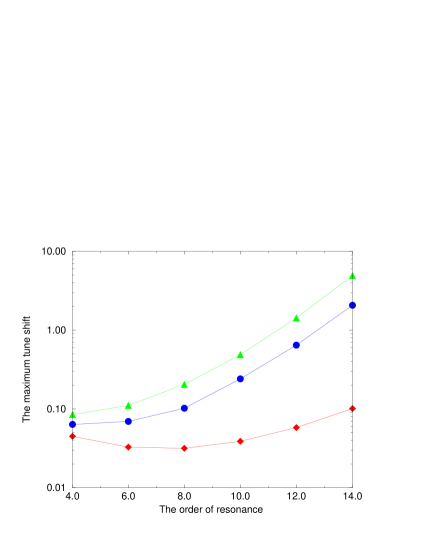
Figure 3: The maximum beam-beam tune shift vs the resonance order. For a flat beam the dotted line and the diamonded line correspond to the horizontal and vertical tune resonances, respectively. The triangled line corresponds to the vertical resonance for a round beam case.

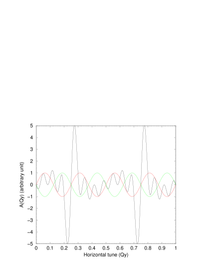
Figure 4: The nonlinear perturbation amplitude vs the vertical tune. The two inversely phased sinusoidal curves correspond to the amplitude of the octupole term, and the fast oscillating curve is the sum of the multipoles of the same amplitude from octupole to 28 poles.

Now we investigate how the order of nonlinear resonance affects the maximum beam-beam tune shift. By using eqs. 44, 42, and 46, and assuming that $\tau_{x}=\tau_{y}$, one gets the maximum beam-beam tune shift with respect to the order of nonlinear resonance, $m$, as shown in Fig. 3, where each maximum beam-beam tune corresponds to each dominating multipole resonance. For flat beams, it is obvious that if the horizontal tune is not well chosen, the $\xi_{y,max}^{FB}$ can be 0.032 instead of 0.0447, however, if the vertical resonances have been successfully avoided before $\xi_{x,FB}$ reaches its limit, one could possibly obtain $\xi_{x,max,FB}(\tau_{bb}=1$ hour)$=0.0632$ even difficultly. What should be stressed is that in choosing the working point in the tune diagram, one has to pay attention to the nonlinear resonances of order as high as 14. To explain qualitatively why the maximum beam-beam tune shifts for both round and flat beams seem to be limited by the lowest order of resonance, i.e., the 1/4 resonance, we have plotted in Fig. 4 the sum of the multipole strengths from m=4 to m=14 assuming that they have the same strength, as expressed:

$$A(Q_{y})=\sum_{m=4}^{m=14}(-1)^{m/2}\sin(2\pi mQ_{y})$$ (49)

On the same figure we have plotted also the first term (octupole) in this summation with two opposite phases as compare references, and it is obvious that except two regions of $Q_{y}$, (0.2 to 0.3) and (0.7 to 0.8), one has always that the amplitude of the sum is almost the same as that of the octupole term, and in this case the dangerous $Q_{y}$ values are 0.225, 0.275, 0.725 and 0.775. Another reason for the lowest resonance dominating is that the lower the resonance order the more stable the resonance facing to the phase perturbations.

Now we discuss briefly the choice of tunes (working point). Limited to one IP and the flat beam case, based on the original work of Bassetti (LNF-135, Frascati, Italy), B. Richter has shown in ref. [22] that the tune should be chosen just above an integer or half integer to make a best use of dynamic beta effect, and this conclusion has been experimentally observed in CESR [23]. Combining this information with what suggested by eq. 49, one concludes that the tune $Q$ should be chosen in the regions (0,0.2) or (0.5,0.7) to obtain a maximum luminosity. If the collision is effectuated with a definite crossing angle some important synchrobetatron nonlinear resonances, such as $3Q_{x}\pm Q_{s}=p$, should be avoided also. More discussions on the crossing angle effects will be given in section 8. Taking CESR and PEP-II for examples, for CESR one finds $Q_{x}=10.523$ and $Q_{y}=9.597$ [23], and for PEP-II the actual operation working points are $Q_{x}=0.610\pm 0.01$ and $Q_{y}=0.580\pm 0.01$ for Low Energy Ring (LER) and $Q_{x}=0.565\pm 0.01$ and $Q_{y}=0.585\pm 0.01$ for High Energy Ring (HER) [24], which in principal consist with our suggestion.

In this paper, under the assumption that the two colliding beams always have the same transverse dimensions, we have arrived at the beam-beam effect determined lifetimes expressed in eqs. 44, 45, and 46. For a given minimum normalized (with respect to the damping time) beam lifetime one gets universal maximum beam-beam tune shift values corresponding to different cases. In a real machine the situation can be more complicated, such as the flip-flop phenomenon which breaks the symmetry assumed above, and in this case one can continue the discussion starting from eqs. 25, 26, and 27 by differentiating $\sigma_{y}$ from $\sigma_{*,y}$, and by replacing $\sigma$, $\sigma_{x}$ by $\Sigma/\sqrt{2}$, $\Sigma_{x}/\sqrt{2}$, respectively, where $\Sigma=\sqrt{\sigma_{*}^{2}+\sigma^{2}}$ and $\Sigma_{x}=\sqrt{\sigma_{*,x}^{2}+\sigma_{x}^{2}}$. We will not, however, continue our discussions in this direction in an exhaustive way.

7 Applications to some machines

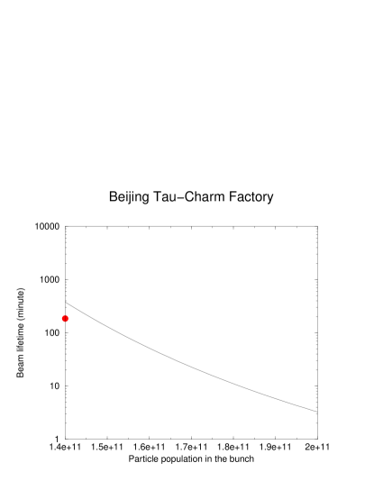
Figure 10: The beam lifetime due to the beam-beam interaction vs the particle population in the bunch in the Beijing $\tau$-C Factory (standard scheme).

Let us look at three machines, PEP-II B-Factory [25] and DA$\Phi$NE [26], and BTCF [27], and the first two have been put to operation. The relevant machine parameters are shown in Table 2. Figs. 5 and 6 give the theoretical estimations for the beam-beam limited beam lifetimes in both PEP-II LER and HER. Figs. 7 and 8 show the beam lifetimes versus the beam-beam tune shifts in both LER and HER. It is obvious that the nominal charge in the bunch of HER is close to the limit which sets the beam lifetime in low energy ring, however, the beam lifetime in HER is much longer than that in LER. The theoretical results consist with the experimental observation [25]. Fig. 9 shows the beam lifetime prediction for the DA$\Phi$NE e⁺e^- collider with single IP. Finally, we study the beam-beam limited beam lifetime in BTCF (standard scheme) and the theoretical result is given in Fig. 10 where the dot indicates the designed beam lifetime.

Machine	$N_{e}$	$\beta_{y,IP}$ cm	$\sigma_{x,IP}$ $\mu$m	$\sigma_{y,IP}$ $\mu$m	$\gamma$	$\tau_{y}$ ms
PEP-II LER	6$\times 10^{10}$	1.5	157	4.78	6067	30
PEP-II HER	2.8$\times 10^{10}$	1.5	157	4.78	17613	18.3
DA$\Phi$NE	8.9$\times 10^{10}$	4.5	2100	21	998	35.7
BTCF	1.4$\times 10^{11}$	1	450	9	3914	31

Table 2: Machine parameters

8 Discussion on the collision with a crossing angle

To get a higher luminosity one could run a circular collider in the multibunch operation mode with a definite collision crossing angle. Different from the head-on collision discussed above, the transverse kick received by a test particle due to the space charge field of the counter rotating bunch will depend on its longitudinal position with respect to the center of the bunch which the test particle belongs to. In this section we consider first a flat beam colliding with another flat beam with a half crossing angle of $\phi$ in the horizontal plane. Due to the crossing angle the two curvilinear coordinates of the two colliding beams at the interaction point will be no longer coincide. The detailed discussion about the coordinates transformation can be found in ref. [28]. When the crossing angle is not too large one has:

$$x^{*}=x+z\phi$$ (50)

where $x^{*}$ is the horizontal displacement of the test particle to the center of the colliding bunch, $z$ and $x$ are the longitudinal and horizontal displacements of the test particle from the center of the bunch to which it belongs. Now we recall eq. 17 which describes the Hamiltonian of the horizontal motion of a test particle in the head-on collision mode, and by inserting eq. 50 into eq. 17 we get:

$$H_{x}={p_{x}^{2}\over 2}+{K_{x}(s)\over 2}x^{2}+{N_{e}r_{e}\over 2\gamma_{*}}({1\over\sigma_{x}^{2}}(x+z\phi)^{2}-{1\over 12\sigma_{x}^{4}}(x+z\phi)^{4}+{1\over 180\sigma_{x}^{6}}(x+z\phi)^{6}$$

$$-{1\over 3360\sigma_{x}^{8}}(x+z\phi)^{8}+\cdot\cdot\cdot)\sum_{k=-\infty}^{\infty}\delta(s-kL)\qquad({\rm FB})$$ (51)

Since the test particle can occupy a definite $z$ within the bunch according to a certain probability distribution, say Gaussian, it is reasonable to replace $z$ in eq. 51 by $\sigma_{z}$, and in this way we reduce a two dimensional Hamiltonian expressed in eq. 51 into a one dimensional one. What should be noted is that eq. 51 takes only the test particle’s longitudinal position into consideration which is regarded as a small perturbation to the head-on collision case, and the geometrical effect will included later. To simplify our analysis we consider only the lowest synchrobetatron nonlinear resonance, i.e., $3Q_{x}\pm Q_{s}=p$ (where $Q_{s}$ is the synchrotron oscillation tune, and $p$ is an integer) which turns out to be the most dangerous one [29][30]. Following the same procedure in section 4 one gets the dynamic aperture due to the lowest synchrobetatron nonlinear resonance as follows:

$$A_{syn-beta,x}(s)=\left({2\beta_{x}(s)\over 3\beta_{x}(s_{IP})^{3}}\right)^{1/2}{2\gamma_{*}\sigma_{x}^{4}\over N_{e}r_{e}\sigma_{z}\phi}$$ (52)

and

$${\cal R}_{syn-beta,x}={A_{syn-beta,x}(s)^{2}\over\sigma_{x}(s)^{2}}={2\over 3\pi^{2}}\left({1\over\xi_{x}^{*}\Phi}\right)^{2}$$ (53)

where $\Phi={\sigma_{z}\over\sigma_{x}}\phi$ is Piwinski angle. Now we are facing a problem of how to combine the two effects: the principal vertical beam-beam effect and the horizontal crossing angle induced perturbation. To solve this problem we assume that the total beam lifetime due to the vertical and the horizontal crossing angle beam-beam effects can be expressed as:

$$\tau_{bb,total}^{*}={\tau_{x}^{*}+\tau_{y}^{*}\over 4}\left({1\over{1\over{\cal R}_{y,8,FB}}+{1\over{\cal R}_{syn-beta,x}}}\right)^{-1}\times$$

$$\exp\left({1\over{1\over{\cal R}_{y,8,FB}}+{1\over{\cal R}_{syn-beta,x}}}\right)\qquad({\rm FB})$$ (54)

where ${\cal R}_{y,8,FB}$ corresponds to eq. 31. After the necessary preparations, we can try to answer two frequently asked questions. Firstly, for a machine working at the head-on collision beam-beam limit, how the beam lifetime depends on the crossing angle? Secondly, for a definite crossing angle, to keep the beam lifetime the same as that of the head-on collision at the beam-beam limit, how much one has to operate the machine below the designed head-on peak luminosity? To answer the first question we define a lifetime reduction factor:

$$R(\Phi)={\tau_{bb,total}^{*}\over\tau_{bb,y}^{*}}\qquad({\rm FB})$$ (55)

where $\tau_{bb,y}^{*}$ is given in eq. 43, and $R(\Phi)$ will tell us to what extent one can increase $\Phi$. Concerning the second question, one can imagine to reduce the luminosity at beam-beam limit by a factor of $f(\Phi)$ in order to against the additional lifetime reduction term due to the definite crossing angle. Physically, from eq. 54 one requires:

$$\left({A_{syn-beta,x}(s)^{2}\over\sigma_{x}(s)^{2}}\right)^{-1}+\left({A_{dyna,crossing,8,y}(s)^{2}\over\sigma_{y}(s)^{2}}\right)^{-1}$$

$$=\left({A_{dyna,head-on,8,y}(s)^{2}\over\sigma_{y}(s)^{2}}\right)^{-1}\qquad({\rm FB})$$ (56)

Mathematically, one has to solve the following equation to find the peak luminosity reduction factor $f(\Phi)$:

$${3\pi^{2}\xi_{x,design,FB}^{2}f(\Phi)^{2}\Phi^{2}\over 2}+{\sqrt{2}\pi\xi_{y,max,FB}f(\Phi)\over 3}={\sqrt{2}\pi\xi_{y,max,FB}\over 3}\qquad({\rm FB})$$ (57)

$$f(\Phi)={-b_{0}+\sqrt{b_{0}^{2}+4a_{0}c_{0}}\over 2a_{0}}\qquad({\rm FB})$$ (58)

where $a_{0}=3\pi^{2}\xi_{x,design,FB}^{2}\Phi^{2}/2$, $b_{0}=c_{0}=\sqrt{2}\pi\xi_{y,max,FB}/3$, and $\xi_{x,max,FB}\approx 0.0447$. In fact, $f(\Phi)$ corresponds to the luminosity reduction due to the synchrobetatron resonance, and to find out the total luminosity reduction factor, one has to include the geometrical effects [31][32]. The total luminosity reduction factor can be expressed as follows:

$$F(\Phi)=f(\Phi)\left(1+\Phi^{2}\right)^{-1/2}\qquad({\rm FB})$$ (59)

where hourglass effect is no taken into account (i.e. $\beta_{y,IP}>\sigma_{z}$). Taking KEKB factory as an interesting example [25], one has $\sigma_{x}=90$ $\mu$m,$\sigma_{z}=0.4$ cm, $\phi=11$ mrad, $\Phi=0.49$, $\xi_{x,design,FB}=0.039$, and by putting $\Phi=0.49$ into eq. 58 one finds $F(0.49)=83.5\%$ which is very close to a three dimensional numerical simulation result, i.e., $85\%$ of designed head-on luminosity, given in ref. [33]. In Figs. 11 and 12 we show how $R(\Phi)$ and $F(\Phi)$ depend on Piwinski angle where $\xi_{x,design,FB}=0.039$ has been used in Fig. 12. Finally, when the crossing angle is in the vertical plane or the beam is round, one gets:

$${\cal R}_{syn-beta,y}={1\over 3\pi^{2}}\left({r\over\xi_{y}^{*}\Phi}\right)^{2}\qquad({\rm FB})$$ (60)

and

$${\cal R}_{syn-beta,y}={32\over 27\pi^{2}}\left({1\over\xi_{y}^{*}\Phi}\right)^{2}\qquad({\rm RB})$$ (61)

where $r=\sigma_{y}/\sigma_{x}$ and $\Phi={\sigma_{z}\over\sigma_{x}}\phi$ as defined before. Replacing ${\cal R}_{syn-beta,x}$ in eq. 54 by eq. 60 or eq. 61 and following the same procedure shown above one can easily make the corresponding discussions on the luminosity reduction effects. What should be remembered is that the geometrical luminosity reduction factors for the vertical crossing angle and the round beam cases are $(1+(\Phi/r)^{2})^{-1/2}$ and $(1+\Phi^{2})$, respectively.

9 Conclusion

In this paper we have established analytical formulae for the beam-beam interaction limited dynamic apertures and beam lifetimes in e⁺e^- circular colliders for both round and flat beam cases. It is shown analytically why for flat colliding beams one has always $\xi_{y,max}$ around 0.045 and why this value can be almost doubled by using round beams. Applications to the machines, such as PEP-II, DA$\Phi$NE, and BTCF have been made. Finally, the luminosity reduction due to a crossing angle has been discussed, and an analytical formula for the luminosity reduction factor is derived and compared with a numerical simulation result for KEKB factory.

10 Acknowledgement

The author thanks J. Haïssinski for his careful reading of the manuscript, critical comments, and drawing my attention to the paper of B. Richter. Stimulating discussions with A. Tkatchenko and J. Le Duff are appreciated.

Figure 1: ${\tau_{bb}^{*}\over\tau_{y}^{*}}$ vs $\xi_{y}^{*}$ for flat beam case.

Figure 2: ${\tau_{bb}^{*}\over\tau_{y}^{*}}$ vs $\xi_{y}^{*}$ for round beam case.

Figure 5: The beam lifetime due to the beam-beam interaction vs the particle population in the bunch in the low energy ring of PEP-II.

Figure 6: The beam lifetime due to the beam-beam interaction vs the particle population in the bunch in the high energy ring of PEP-II.

Figure 7: PEP-II Low Energy Ring (flat beam): the beam-beam limited lifetime $\tau_{bb}^{*}$ (hours) vs the vertical beam-beam tune shift $\xi_{y}$.

Figure 8: PEP-II Low Energy Ring (round beam is assumed): the beam-beam limited lifetime $\tau_{bb}^{*}$ (hours) vs the vertical beam-beam tune shift $\xi_{y}$.

Figure 9: The beam lifetime due to the beam-beam interaction vs the particle population in the bunch in the DA$\Phi$NE $\Phi$-Factory.

Figure 11: The lifetime reduction factor $R(\Phi)$ vs Piwinski angle $\Phi$.

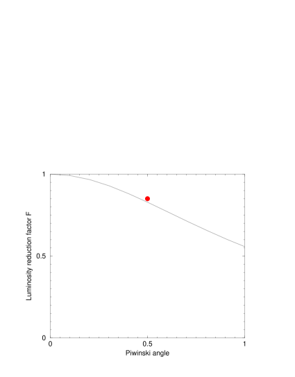
Figure 12: The luminosity reduction factor $F(\Phi)$ vs Piwinski angle $\Phi$. The curve is obtained by taking $\xi_{x,design,FB}=0.039$ (KEKB), and the dot is the numerical simulation result given in ref. [33].

References

• [1] J. Gao, “Analytical estimation of the dynamic apertures of circular accelerators”, Nucl. Instr. and Methods, A451 (3) (2000), p. 545.
• [2] A. Piwinski, “Observation of beam-beam effects in PETRA”, IEEE Trans. on Nucl. Science, Vol. NS-26, No. 3, June 1979.
• [3] M.A. Furman, “Beam-beam issues for high luminosity e+e- colliders”, Frascati physics series Vol. X (1998), p. 123.
• [4] E. Keil, “Beam-beam dynamics”, CERN 95-06, p. 539.
• [5] R. Talman, “Resonances in accelerators”, AIP Conference Proceedings 153 (1984), p. 835.
• [6] T. Chen, J. Irwin, and R.H. Siemann, “High-order horizontal resonances in the beam-beam interaction”, Nucl. Instr. and Methods, A402 (1998), p. 21.
• [7] S. G. Peggs and R. M. Talman, “Nonlinear problems in accelerator physics”, Ann. Rev. Nucl. Part. Sci. Vol. 36 (1986), p. 287.
• [8] S. Peggs and R. Talman, “Beam-beam luminosity in electron-positron colling rings”, Physical Review D, Vol 24, No.9 (1981), p. 2379.
• [9] A. Chao and M. Tigner (Editors), “Handbook of accelerator physics and engineering”, World Scientific (1999), p. 134.
• [10] M. Bassetti and G. Erskine, “Closed expression for the electrical field of a two-dimensional Gaussian charges”, CERN/ISR-TH/80-06 (1980).
• [11] V. Ziemann, “Beyond Bassetti and Erskine: beam-beam deflections for non-Gaussian beams”, SLAC-PUB-5582 (1991).
• [12] R. Talman, “Multiparticle phenomena and Landau damping”, AIP Conference Proceedings 153 (1984), p. 790.
• [13] K. Hirata, “The beam-beam interaction: Coherent effects”, AIP Conference Proceedings 214 (1990), p. 175.
• [14] K. Hirata, “Coherent betatron oscillation modes due to beam-beam interaction”, Nucl. Instr. and Methods, A269 (1988), p. 7.
• [15] K. Hirata and E. Keil, “Barycentre motion of beams due to beam-beam interaction in asymmetric ring colliders”, Nucl. Instr. and Methods, A292 (1990), p. 156.
• [16] S. Krishnagopal and R. Siemann, “A comparison of fat beams with round”, AIP Conference Proceedings 214 (1990), p. 278.
• [17] S. Krishnagopal and R. Siemann, “Simulation of round beams”, PAC89, p. 836.
• [18] M. Bassetti and M.E. Biagini, “A beam-beam tune shift semi-empirical fit”, Frascati physics series Vol. X (1998), p. 289.
• [19] J. Gao, “Analytical formulae for the maximum beam-beam tune shift in electron storage rings”, Nucl. Instr. and Methods, A413 (1998), p. 431.
• [20] J. Gao, “Analytical formulae for the maximum beam-beam tune shift in circular colliders”, LAL-SERA-99-148.
• [21] H. Bruck, “Accélérateurs circulaires de particules” (Press Universitaires de France, 1966, p. 268.
• [22] B. Richter, “Design considerations for high energy electron-positron storage rings”, Proceedings of the international symposium on electron-positron circular colliders”, 26-30 September, 1966, Saclay, France, p. I-1-1.
• [23] D. Sagan, “The dynamic beta effect in CESR”, Proceedings of PAC95, USA (1995), p. 2889.
• [24] M. Placidi, “Beam-beam issues from the recent PEP-II commissioning”, Proceedings of workshop on beam-beam effects in large hadron colliders, CERN, 1999, p. 45.
• [25] J.T. Seeman, “Commissioning results of the KEKB and PEP-II B-factories”, PAC99, New York, 1999, p. 1.
• [26] G. Vignola, “DA$\Phi$NE, the Frascati $\Phi$-factory”, PAC93, USA (1993),p. 1993.
• [27] “Feasibility study report on Bejing Tau-Charm Factory”, IHEP-BTCF Report-01, Dec. 1995.
• [28] K. Hirata, “Analysis of beam-beam interactions with a large crossing angle”, Physical Review Letters, Vol. 74, No. 12, March 1995, p. 2228.
• [29] A. Piwinski, “Satellite resonances due to beam-beam interaction”, IEEE Trans. on Nucl. Sci., Vol. NS-24, No. 3, June 1977, p. 1408.
• [30] A. Piwinski, Computer simulation of the beam-beam interaction at a crossing angle”, IEEE Trans. on Nucl. Sci., Vol. NS-32, No. 5, Oct. 1985, p. 2240.
• [31] A. Piwinski, “Satellite resonances due to beam-beam interaction”, Nucl. Instr. and Methods, 81 (1970), p. 199.
• [32] N. Toge and K. Hirata, “Study on beam-beam interactions for KEKB”, KEK Preprint 94-160.
• [33] K. Ohmi, “Simulation of the beam-beam effect in KEKB”, KEK proceedings 99-24, p. 187 (International workshop on performance improvement of electron-positron collider particle factories).
Refer to caption