Abstract

Our theoretical comparisons suggest that the ATF measurement results of April 2000 for energy spread, bunch length, and horizontal emittance vs. current, and a low current emittance ratio of about 1% are generally consistent with intrabeam scattering (IBS) theory, though the measured effects appear to be stronger than theory. In particular, the measured factor of 3 growth in vertical emittance at 3 mA does not seem to be supported. It appears that either (1) there is another, unknown force in addition to IBS causing emittance growth in the ATF; or (2) the factor of 3 vertical emittance growth is not real, and our other discrepancies are due to the approximate nature of IBS theory. Our results suggest, in addition, that, even if IBS theory has inaccuracies, the effect will be useful as a diagnostic in the ATF. For example, by measuring the energy spread, one will be able to obtain the emittances. Before this can be done, however, more benchmarking measurements will be needed.

Intrabeam Scattering Analysis of ATF Beam Data Taken in April 2000

Introduction

Between April 13-19, 2000 single bunch energy spread, bunch length, and horizontal and vertical emittances in the ATF were all measured as a function of current[1]-[3]. One surprising outcome was that the vertical emittance appeared to grow by a factor of 3 by a current of 3 mA. The ATF is a prototype damping ring for the JLC/NLC linear colliders, and the concern with this result is that it may portend an as yet not understood and unexpected growth in such damping rings, which would have negative ramifications on collider performance. However, since the $x$-$y$ coupling in the ATF is very small ($\sim 1\%$), and since the emittance measurements were performed on the beam after it had been extracted from the ring, the question was, How much of this measured $y$-emittance growth was real and how much was due to measurement error, such as dispersion in the extraction line or in the wire monitors used for the measurements.

With the ATF as it is now, running below design energy and with the wigglers turned off, the beam properties are strongly affected by intra-beam scattering (IBS), an effect that couples the three dimensions of the beam together. In April 2000 all the beam dimensions were measured to varying degrees of accuracy, and the hope is that the knowledge of IBS theory can be used to check for consistency in the data. Besides the question of the vertical emittance growth, we hope that IBS theory can be used in beam diagnostics in the future. For example, the energy spread measurement is quick, accurate, and easy to do. It would be nice if this measurement could be used to estimate the beam emittance and/or bunch length, beam properties that are much more difficult to measure directly.

The literature on intrabeam scattering is quite extensive. (For an introduction, see for example the IBS section and its bibliography, written by A. Piwinski, in the Handbook of Accelerator Physics and Engineering  [4]). The first rather thorough treatment of IBS in circular accelerators is due to Piwinski (P), derived following a two-particle Coulomb scattering formalism[5]. Another formalism is that of Bjorken-Mtingwa (B-M), obtained following quantum mechanical two particle scattering rules[6]. This is the formalism that is more often used in modern optics programs that also calculate IBS, programs such as SAD[7]. The B-M result is considered to be more general in that the combination of optics terms $\beta_{x}\phi_{x}\equiv(\beta_{x}\eta_{x}^{\prime}-\beta_{x}^{\prime}\eta_{x}/2)$ around the ring do not need to be small compared to $\eta_{x}$, whereas in the P method it seems they do[8]. (Note that this condition is typically violated in modern low emittance storage rings.) The B-M formalism, however, does not include vertical dispersion, whereas the P formalism does. Neither formalism includes $x$-$y$ coupling, though a more generalized formulation, which includes both linear coupling and can also be applied to low emittance machines, is given by Piwinski in Ref. [9]. Note that in deriving such formulations many approximations were made, having to do with the cut-off distance for scattering (typically taken to be the vertical beam size), curved trajectories, etc. In addition, it appears that no current IBS formalism properly accounts for the effects of potential well distortion or of the micro-wave instability. Finally, T. Raubenheimer has pointed out that IBS does not result in Gaussian bunch distributions, and that these theories give rms beam sizes that can greatly overemphasize few particles occupying the tails[10].

Most of the early papers comparing IBS theory and measurement were for bunched and unbunched hadronic machines, where the effect tends to be more pronounced than in high energy electron machines. For example, Conte and Martini, for unbunched protrons in the CERN Antiprotron Accumulator ring, found good agreement for the longitudinal and horizontal IBS growth rates, but no agreement for the vertical rate[11]. Evans and Gareyte, for bunched protrons in the SPS, found good agreement for the radial emittance growth rate with time, once an additional factor representing gas scattering was included[12]. As for electron machines, both IBS and the related Touschek effect have become important effects in modern, low emittance light sources. C.H. Kim at the ALS found that he can get agreement with measured horizontal emittance growth with current, but to do this he needed to include a significant additional fitting factor in the calculations[13]. So it may be too much to expect good agreement between IBS theory and measurement without the use of such fudge factors. Indeed, A. Piwinski has said that, given the approximations taken in deriving IBS theory, one can expect agreement between theory and measurement only on the order of a factor of 2[8]. Yet even if this became the case, it may still be possible to benchmark the ATF with accurate emittance and energy spread measurements, to find the fudge factors. Then in the future, one may be able to perform simpler measurements—like the energy spread measurement—to get an estimate of parameters that are more difficult to obtain directly, such as bunch length and emittance.

Piwinski’s Solution

We are interested in what happens at low coupling, and we will concentrate on using the more simplified version of Piwinski’s solution. We begin by reproducing the Piwinski solution in its entirety[4]. Note that there is nothing new in this section, except the way potential well distortion is added to the calculation.

Let us consider the IBS growth rates in energy $p$, in the horizontal direction $x$, and in the vertical direction $y$ to be defined as

$${1\over T_{p}}={1\over\sigma_{p}}{d\sigma_{p}\over dt}\ ,\quad{1\over T_{x}}={1\over\epsilon_{x}^{1/2}}{d\epsilon_{x}^{1/2}\over dt}\ ,\quad{1\over T_{y}}={1\over\epsilon_{y}^{1/2}}{d\epsilon_{y}^{1/2}\over dt}\ .$$ (1)

Here $\sigma_{p}$ is the rms (relative) energy spread, $\epsilon_{x}$ the horizontal emittance, and $\epsilon_{y}$ the vertical emittance. According to Piwinski the IBS growth rates are given as

$${1\over T_{p}}=\left<A{\sigma_{h}^{2}\over\sigma_{p}^{2}}f(a,b,q)\right>$$ (2)

$${1\over T_{x}}=\left<A\left[f({1\over a},{b\over a},{q\over a})+{D_{x}^{2}\sigma_{h}^{2}\over\sigma_{x\beta}^{2}}f(a,b,q)\right]\right>$$ (3)

$${1\over T_{y}}=\left<A\left[f({1\over b},{a\over b},{q\over b})+{D_{y}^{2}\sigma_{h}^{2}\over\sigma_{y\beta}^{2}}f(a,b,q)\right]\right>$$ (4)

where the brackets $\langle\rangle$ mean that the enclosed quantities, combinations of beam parameters and lattice properties, are averaged around the entire ring. Parameters are:

$$A={r_{0}^{2}N\over 64\pi^{2}\beta^{3}\gamma^{4}\epsilon_{x}\epsilon_{y}\sigma_{s}\sigma_{p}}$$ (5)

$${1\over\sigma_{h}^{2}}={1\over\sigma_{p}^{2}}+{D_{x}^{2}\sigma_{h}^{2}\over\sigma_{x\beta}^{2}}+{D_{y}^{2}\sigma_{h}^{2}\over\sigma_{y\beta}^{2}}$$ (6)

$$a={\sigma_{h}\beta_{x}\over\gamma\sigma_{x\beta}},\quad b={\sigma_{h}\beta_{y}\over\gamma\sigma_{y\beta}},\quad q=\sigma_{h}\beta\sqrt{{2d\over r_{0}}};$$ (7)

The function $f$ is given by:

$$f(a,b,q)=8\pi\int_{0}^{1}\left\{2\ln\left[{q\over 2}\left({1\over P}+{1\over Q}\right)\right]-0.577\ldots\right\}{1-3u^{2}\over PQ}\,du$$ (8)

$$P^{2}=a^{2}+(1-a^{2})u^{2},\quad\quad Q^{2}=b^{2}+(1-b^{2})u^{2}$$ (9)

The global beam properties that are affected by IBS are the rms (relative) energy spread $\sigma_{p}$ and the rms bunch length $\sigma_{s}$, the horizontal emittance $\epsilon_{x}$, and the vertical emittance $\epsilon_{y}$. Other global properties are the bunch population $N$, the relative velocity $\beta$, and the energy factor $\gamma$. Note that $r_{0}$ is the classical radius of the particles (for electrons $r_{0}=2.82\times 10^{-15}$ m). The lattice functions needed are the beta functions $\beta_{x}$, $\beta_{y}$, and the dispersion functions $D_{x}$, $D_{y}$. Note also that $\sigma_{x\beta}=\sqrt{\beta_{x}\epsilon_{x}}$, and $\sigma_{y\beta}=\sqrt{\beta_{y}\epsilon_{y}}$. The parameter $d$ represents a cut-off for the IBS force, which Piwinski says should be taken as the vertical beam size, but he also points out that the results are not very sensitive to exactly what is chosen for this parameter.

Then the steady-state beam properties are given by

$$\epsilon_{x}={\epsilon_{x0}\over 1-\tau_{x}/T_{x}}\ ,\ \epsilon_{y}={\epsilon_{y0}\over 1-\tau_{y}/T_{y}}\ ,\ \sigma^{2}_{p}={\sigma^{2}_{p0}\over 1-\tau_{p}/T_{p}}\ ,$$ (10)

where subscript 0 represents the beam property due to synchrotron radiation alone, i.e. in the absence of IBS, and $\tau_{x}$, $\tau_{y}$, and $\tau_{p}$ are the synchrotron radiation damping times in the three directions. These are 3 coupled equations in that all 3 IBS rise times depend on $\epsilon_{x}$, $\epsilon_{y}$, and $\sigma_{p}$. Note that a 4th equation, the relation between $\sigma_{s}$ and $\sigma_{p}$, is also implied; generally this is taken to be the nominal (zero current) relationship.

Piwinski suggests iterating Eqs. 10 until a self-consistent solution is found. Our experience is that this has the problem that negative values of emittance or $\sigma_{p}^{2}$ can be obtained with this procedure, causing difficulty in knowing how to continue the iteration. We find that a better method is to convert these equations into 3 coupled differential equations, such as is done in Ref. [13] to obtain the time development of the beam properties in a ring. Here, however, we use it only as a mathematical device for finding the steady-state solution. For example, the equation for $\epsilon_{x}$ becomes

$${d\epsilon_{x}\over dt}=-{(\epsilon_{x}-\epsilon_{x0})\over\tau_{x}}+{\epsilon_{x}\over T_{x}}\quad,$$ (11)

and there are corresponding equations for $\epsilon_{y}$ and $\sigma_{p}^{2}$.

We have three comments: (1) In a storage ring vertical emittance is generally the result of two phenomena, $x$-$y$ coupling—caused, for example, by rolled magnets—and vertical dispersion—caused by vertical closed orbit distortion. Although our formalism technically is valid only for the case of no $x$-$y$ coupling, we believe that it can also be used for the case of weak coupling. In such a case we simply pick a zero-current emittance ratio $r_{xy0}=\epsilon_{y0}/\epsilon_{x0}$, and then set $\epsilon_{y0}$ accordingly. Note that $r_{xy0}$ is meant to include both the contributions of $x$-$y$ coupling and of vertical dispersion. Finally, note that the vertical emittance, assuming only vertical dispersion, can be approximated by[14]

$$\epsilon_{y0}=2{\cal J}_{\epsilon}{(D_{y})_{rms}^{2}\over\langle\beta_{y}\rangle}\sigma_{p0}^{2}\quad,$$ (12)

with ${\cal J}_{\epsilon}$ the energy damping partition number.

(2) It is not clear how impedance effects and IBS effects interact. At the ATF we have shown that up to the currently highest attainable single bunch currents ($\sim 3$ mA) a micro-wave threshold has not yet been reached[1]. But we do appear to have a sizeable potential well bunch lengthening effect. We will assume that this case can be approximated by adding the proper multiplicative factor $f_{pw}(N)$, obtained from measurements, to the equation giving $\sigma_{s}$ in terms of $\sigma_{p}$. (3) As mentioned earlier, the IBS bunch distributions are not Gaussian, and tail particles can be overemphasized in the beam size solutions given above. T. Raubenheimer in Ref. [10] gives a way of estimating IBS beam sizes that better reflect the particles in the core of the beam. Note that the optics computer program SAD can solve the IBS equations of B-M, include the effects of orbit errors, and also find the sizes of the core of the beam.

Parameter Studies

We have programmed the above Piwinski equations. We have also programmed the B-M equations, which also give 3 IBS growth rates (though there is a factor of 2 difference in their definition). Let us begin our numerical studies by comparing the results of the two programs when applied to the ATF lattice and beam properties. (Note that there is a published comparison of results of these two methods applied to the CERN AA ring in Ref. [15]; however, the variation of the lattice parameters around the ring was not included in the P method calculation.) As parameters we take: $E=1.28$ GeV, $\sigma_{p0}=5.44\times 10^{-4}$, $\sigma_{s0}=5.06$ mm (for an rf voltage of 300 kV), $\epsilon_{x0}=1.05$ nm, $\tau_{p}=20.9$ ms, $\tau_{x}=18.2$ ms, and $\tau_{x}=29.2$ ms. The ATF circumference is 138 m, $\langle\beta_{x}\rangle=4.2$ m, $\langle\beta_{y}\rangle=4.6$ m, $\langle D_{x}\rangle=5$ cm. The function $\beta_{x}|\phi_{x}|$ is about $.5D_{x}$ at positions of the minima in $D_{x}$, and about $.15D_{x}$ at positions of the maxima, which are not so small, and we might expect some disagreement between the two methods. Note that for the averages represented by brackets in Eqs. 2-4, and their counterparts in the B-M method, we calculate, as is normally done, the appropriate combination of lattice and beam properties at the ends of the lattice elements, connect these with straight lines, and then find the average of the resulting curve.

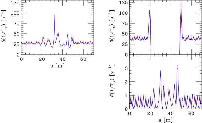
Figure 1: Differential growth rates over 1/2 the ATF, as obtained by the Piwinski (blue) and the Bjorken-Mtingwa (red) methods Here $I=3.1$ mA, $r_{xy0}=.01$, and $D_{y}=0$ (no vertical dispersion).

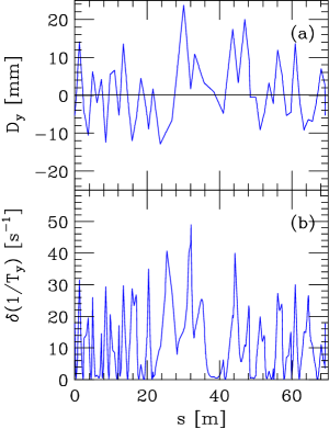
Figure 2: Random vertical dispersion [$(D_{y})_{rms}=7.5$ mm] (a), and the resulting differential vertical growth rate (b) over 1/2 the ATF. $1/T_{y}=11.8$ s^-1. Here $I=3.1$ mA and $r_{xy0}=.01$.

Fig. 1 displays the 3 differential IBS growth rates as obtained by the two methods (blue for P, red for B-M) when $I=3.1$ mA and $r_{xy0}=.01$. The IBS growth rates are just the average values over the ring of these functions. Since the ATF has two-fold symmetry we give the result for only half the ring (the straight section is in the middle). Here we include no vertical dispersion, i.e. the vertical emittance is presumed to be only due to (weak) $x$-$y$ coupling, and $f_{pw}$ is set to 1. We see almost perfect agreement for the differential growth rates obtained by the two methods, with only slight differences in the peaks. As for the averages, for the Piwinski method $1/T_{p}=28.4$ s^-1, $1/T_{x}=24.8$ s^-1, and $1/T_{y}=.67$ s^-1. The B-M results are 28.9, 26.2, and .58 s^-1, respectively. Note that the $y$ growth rates are very small. As for the steady state beam properties, for this example $\sigma_{p}/\sigma_{p0}=1.566$, $\epsilon_{x}/\epsilon_{x0}=1.825$, and $\epsilon_{y}/\epsilon_{x0}=.0102$ for P, and 1.587, 1.910, .0102 for B-M, respectively. We see that for the ATF the results of the two methods are almost the same. Finally, note that when making the same comparison for the ALS at Berkeley, a low emittance light source with $\beta_{x}|\phi_{x}|$ comparable to $D_{x}$, we again find very close agreement in the results of the two methods.

In the ATF the rms vertical dispersion, after correction, is typically 3-4 mm. To simulate this effect we added a randomly generated component of $D_{y}$ (weighted by $\sqrt{\beta_{y}}$) at the high and low $\beta_{y}$ points, and connected these with straight lines (see Fig. 2a). This was added to the P calculation. In the ATF typically $r_{xy0}\approx.01$ and ${\cal J}_{\epsilon}=1.4$. We see from Eq. 12 that if $(D_{y})_{rms}=4$ mm, then 30% of the low current emittance is due to dispersion, and the rest due to $x$-$y$ coupling. Let us consider an example now where the size of $\epsilon_{y0}$ is given entirely by vertical dispersion, with $r_{xy0}=.01$ and $(D_{y})_{rms}=7.5$ mm. In Fig. 2b we plot the resulting $\delta(1/T_{y})$ at $I=3.1$ mA. The growth is much larger than before, with $1/T_{y}=11.8$ s^-1. (Note that $\sigma_{p}/\sigma_{p0}=1.48$, $\epsilon_{x}/\epsilon_{x0}=1.71$, and $\epsilon_{y}/\epsilon_{x0}=.015$.) We can understand the change in $1/T_{y}$ if we look back at the equations for the growth rates in $x$ and $y$, Eqs. 3 and 4. In Eq. 3 the horizontal growth rate is dominated by the second term in the brackets, the one proportional to $D_{x}^{2}/\sigma_{x\beta}^{2}$. In Eq. 4 the vertical growth rate, when $D_{y}=0$, is given by the small first term in the brackets. Since the second term is proportional to $D_{y}^{2}/\sigma_{y\beta}^{2}$, $1/T_{y}$ will become comparable to $1/T_{x}$ when $(D_{y})_{rms}\sim\langle D_{x}\rangle\sqrt{\epsilon_{y}/\epsilon_{x}}$ (since $\langle\beta_{x}\rangle$ and $\langle\beta_{y}\rangle$ are similar), which equals 5 mm. Note that the importance grows as the second power of $(D_{y})_{rms}$.

We see that the Piwinski and the Bjorken-Mtingwa methods give essentially the same solution for the ATF, and since the P method allows for vertical dispersion, we will choose to continue our simulations using this method. In Figs. 3-5 we give the steady-state emittance and energy spread vs. various parameters in the ATF according to Piwinski’s IBS theory. We include curves representing $(D_{y})_{rms}=0$, 3, and 6 mm. [Note that $(D_{y})_{rms}=0$ is not a realistic condition for the ATF.] Given the approximate nature of IBS theory, these results are meant to give an idea of the sensitivities of the steady-state beam properties to various parameters, and not to give absolutely correct predictions. In Fig. 3 we show the dependence on $I$, with $f_{pw}=1$, $r_{xy0}=.01$. We note that the vertical emittance growth is almost zero with zero vertical dispersion. At $(D_{y})_{rms}=6$ mm, $\epsilon_{y}$ has increased by 44% by $I=3$ mA. In Fig. 4 we show the dependence on $r_{xy0}$, with $f_{pw}=1$, $I=3.1$ mA. We note that at $r_{xy0}=0$ the vertical emittance does not go to zero when $(D_{y})_{rms}$ is not zero. Note also that for the case $(D_{y})_{rms}=6$ mm, the $\sigma_{p}(r_{xy0})$ curve is rather linear over the range shown, with a slope $\Delta\sigma_{p}/\sigma_{p}/\Delta r_{xy0}=6.6$; i.e. an (absolute) change in $r_{xy0}$ of 0.005 produces a relative change in $\sigma_{p}$ of only 3%. In Fig. 5 we give the dependence on $f_{pw}$, with $I=3.1$ mA, $r_{xy0}=.01$. Note that at $I=3$ mA, the ATF measurements give $f_{pw}=1.25$. We see that the energy spread and emittances are not very sensitive to this parameter. For example, a change of .1 in $f_{pw}$ yields a 1% change in $\sigma_{p}$.

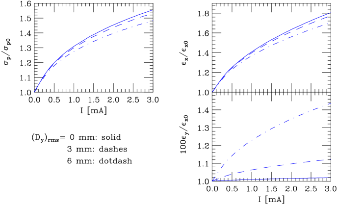
Figure 3: Calculations of the current dependence of the beam properties when $r_{xy0}=.01$, $f_{pw}=1$.

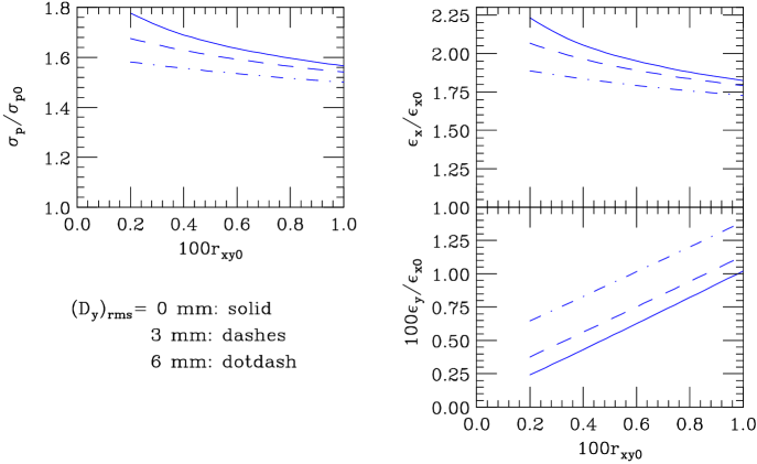
Figure 4: Calculations of the $r_{xy0}$ dependence of the beam properties when $I=3.1$ mA, $f_{pw}=1$.

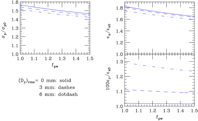
Figure 5: Calculations of the $f_{pw}$ dependence of the beam properties when $I=3.1$ mA, $r_{xy0}=.01$.

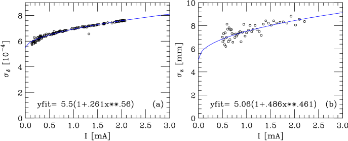
Figure 6: Measurements of energy spread (a) and bunch length (b), with $V_{c}=300$ kV, performed on April 13-14, 2000. The fits (the curves) are chosen to give the expected zero current results.

Measurements[1]-[3]

In April 2000, $\sigma_{p}$, $\sigma_{s}$, $\epsilon_{x}$, and $\epsilon_{y}$ were all measured as functions of current to varying degrees of accuracy. Among the most accurate is believed to be the energy spread measurement, which is performed on a thin screen at a high dispersion region in the extraction line ($D_{x}=1.73$ m). At different currents the measured beam width was fit to a Gaussian (the fits were very good) and the rms width was extracted. This measurement was performed on April 14 (see Fig. 6a). The rms scatter in the extracted $\sigma_{p}$ was less than 2%, and the precision should be better than 1%. Note that although data was obtained for currents up to $\sim 2$ mA only, from experience we have confidence that we can extrapolate to $\sim 3$ mA.

The rms bunch length, using a streak camera, was also measured about the same time, and there was more scatter in the data(see Fig. 6b). With streak camera measurements, however, there is always the question of whether space charge in the streak camera itself could have added a systematic error to the results. Checks were made with light filters, so we don’t think this is a problem, but this still adds a slight uncertainty to the results. Both results were fit to a smooth curve, chosen to give the expected zero current results (see Fig. 6). Note that these results, if true, imply an extremely large bunch length increase at low currents.

The emittances were measured on wire monitors in the extraction line on April 19. The results are reproduced by the plotting symbols in Fig. 7b-c. We see that the $x$ emittance appears to grow by $\sim 80\%$ by $I=3$ mA; the $y$ emittance begins at about 1% of the $x$ emittance, and then grows by a factor of 3. We believe that the $x$-emittance measured should be fairly accurate. The $y$-emittance, however, since it is so small, could be corrupted by many factors, such as dispersion in the extraction line or the wire monitors (roll of the measurement wires, for example, has been checked and shown not to be significant). Note that it appears that $r_{xy0}\sim.01$. We estimated above, using Eq. 12, that if the vertical emittance is dominated by vertical dispersion, then $r_{xy0}=.01$ implies that $(D_{y})_{rms}=7.5$ mm, which is significantly larger than the measured 3-4 mm. Unfortunately, we do not know what $D_{y}(s)$ was during the April measurements, and therefore cannot make a more precise comparison with calculation.

Note that all the measurements were not performed on the same day, and since IBS depends on the status of the machine (e.g. on the vertical closed orbit distortion), it is possible that the longitudinal and transverse measurements correspond to slightly different machines as far as IBS is concerned. For example, on April 13, the day before the $\sigma_{p}$ measurements of Fig. 6, the energy spread was also measured. Those results, when fitted and extrapolated to $I=3$ mA, gave a 2% smaller rms value than given here. This adds some uncertainty to our results.

Comparison with IBS Theory

To study the consistency of these measurements with IBS theory, we perform IBS calculations where we take the potential well factor $f_{pw}$ that was measured, and adjust $r_{xy0}$ to obtain the measured $\sigma_{p}$ (and $\sigma_{s}$) at $I=3$ mA, for the cases $(D_{y})_{rms}=3$ and 6 mm. [Remember: the typical measured value is $(D_{y})_{rms}=3$-4 mm.] The best fits were found for $r_{xy0}=.0104$ and .006, for the cases $(D_{y})_{rms}=3$ and 6 mm, respectively. The results are shown in Fig. 7, where they are compared to the measured data. (Note that in Fig. 7a, we reproduce, using plotting symbols, the smooth curve fits to the measured data of Fig. 6.)

We first notice that whether there is a 3 mm or 6 mm $y$ dispersion the fitted results are very similar. We find for our fitted results that the $\epsilon_{x}$ dependence on current is in reasonable agreement with measurement (though the calculated result is low by 10% at 3 mA), and that $r_{xy0}\sim.006$-.01, which is a little low compared to .01. The biggest discrepancy, however, seems to be that the vertical emittance growth is much lower for the calculations than the measurements: for the case $(D_{y})_{rms}=3$ mm we see 10% growth by 3 mA; for $(D_{y})_{rms}=6$ mm we see 60% growth by 3 mA, which, however, is not close to the factor of 3 that was measured.

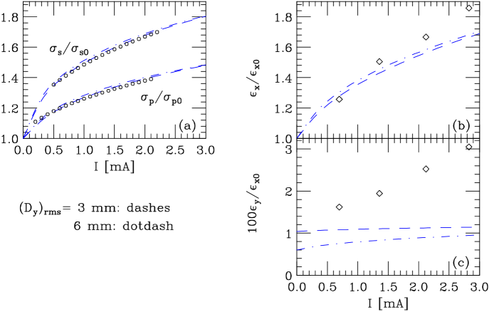
Figure 7: ATF measurement data (symbols) and IBS theory fits (the curves). The symbols in (a) give the smooth curve fits to the measured data of Fig. 6. In the theory the parameter $r_{xy0}$ was adjusted to get the measured $\sigma_{p}$ at $I=3$ mA.

Let us suppose that the measured vertical emittance growth is not real, and is due to measurement error. In such a case, our results appear to give reasonable agreement between IBS theory and the ATF measurements, for $\sigma_{p}$, $\sigma_{s}$, and $\epsilon_{x}$ vs. $I$, and low current $\epsilon_{y}$, all without extra fudge factors. For the present set of data, however, we are still left with some uncertainties. For example, it was suggested earlier that the accurate knowledge of $\sigma_{p}(I)$ is important. It was shown that for a realistic type of vertical dispersion for the ATF, $(D_{y})_{rms}=6$ mm, at $I=3.1$ mA, a change in $r_{xy0}$ of .005 produces a relative change in $\sigma_{p}$ of only 3%. Or, conversely, if the inaccuracy in $\sigma_{p}(3~{}mA)$ is 3%, then the fitted $r_{xy0}$ shifts by .005, which is not small compared to .01. And from the measured difference in $\sigma_{p}$ on April 13 and 14, it seems that the uncertainty in $\sigma_{p}$ is of this order. Finally, we should note that another source of uncertainty is that we don’t know the function $D_{y}(s)$ on the date of the measurements.

However, there is one major quantative discrepancy between theory and measurement, which has to do with non-Gaussian beam tails. SAD finds that for the ATF the IBS induced emittance growth, when not counting such tail particles, is only 2/3 of that when all particles are included (or 80% in the case of $\sigma_{p}$), in agreement with calculations for the ATF given in Ref. [10]. Our calculations include all beam particles, while the measurements consider only core particles. If the tail particles are indeed as significant as these results suggest, then the effect measured at the ATF is much stronger than predicted by IBS theory, and there would no longer be good agreement with measurement. If one wants to think about a fudge factor that is multiplied with the bunch charge, then we estimate that this factor must be $\sim 1.5$-2.0 (though no single such factor gives good agreement for all $\sigma_{p}(I)$, $\sigma_{s}(I)$, and $\epsilon_{x}(I)$). From this result, it appears that either there is another, unknown force in addition to IBS causing emittance growth in the ATF, or the problem is the approximate nature of IBS theory.

In spite of this discrepancy, we believe that the IBS effect will be useful as a diagnostic at the ATF. However, before we can use it as such, we need to perform more benchmarking experiments. Such measurements include the effects of varying the rf voltage, the vertical dispersion, and the $x$-$y$ coupling. Additional independent measurements are also desireable, such as using the interferometer to measure the beam sizes in the ring. The calculations can also be improved by including a cut-off for the tails. In addition, one might, for example, include the measured vertical dispersion (instead of a randomly generated one) and/or use Piwinski’s more involved formulation that properly includes linear coupling.

Conclusion

Our theoretical comparisons suggest that the ATF measurement results of April 2000 for energy spread, bunch length, and horizontal emittance vs. current, and a low current emittance ratio of about 1% are generally consistent with intrabeam scattering (IBS) theory, though the measured effects appear to be stronger than theory. In particular, the measured factor of 3 growth in vertical emittance at 3 mA does not seem to be supported. It appears that either (1) there is another, unknown force in addition to IBS causing emittance growth in the ATF; or (2) the factor of 3 vertical emittance growth is not real, and our other discrepancies are due to the approximate nature of IBS theory. Our results suggest, in addition, that, even if IBS theory has inaccuracies, the effect will be useful as a diagnostic in the ATF. For example, by measuring the energy spread, one will be able to obtain the emittances. Before this can be done, however, more benchmarking measurements will be needed.

References

- [1] K. Bane, et al, “Bunch Length Measurements at the ATF Damping Ring in April 2000,” ATF-00-11, September 2000.
- [2] “ATF (Accelerator Test Facility) Study Report JFY 1996-1999,” KEK Internal 2000-6, August 2000.
- [3] J. Urakawa, Proc. EPAC2000, Vienna (2000) p. 63, and KEK-Preprint 2000-67, August 2000.
- [4] A. Chao and M. Tigner, eds., Handbook of Accelerator Physics and Engineering (World Scientific, 1999) p. 125.
- [5] A. Piwinski, Proc. 9th Int. Conf. on High Energy Acc., Stanford (1974) p. 405.
- [6] J.D. Bjorken and S.K. Mtingwa, Particle Accelerators 13 (1983) 115.
- [7] K. Oide, SAD User’s Guide.
- [8] A. Piwinski, private communication.
- [9] A. Piwinski, “Intrabeam Scattering” in CERN Accelerator School (1991) p. 226.
- [10] T. Raubenheimer, Particle Accelerators 45 (1994) 111.
- [11] M. Conte and M. Martini, Particle Accelerators 17 (1985) 1.
- [12] L.R. Evans and J. Gareyte, PAC85, IEEE Trans. in Nuclear Sci. NS-32 No. 5 (1985) 2234.
- [13] C.H. Kim, “A Three-Dimensional Touschek Scattering Theory,” LBL-42305, September 1998.
- [14] T. Raubenheimer, “The Generation and Acceleration of Low Emittance Flat Beams for Future Linear Colliders,” PhD Thesis, SLAC-387, 1991.
- [15] M. Martini, “Intrabeam Scattering in the ACOL-AA Machines,” CERN PS/84-9 (AA), May 1984.