Cooling gases with Lévy flights:
using the generalized central limit theorem
in physics

Institut de Physique et de Chimie des Matériaux de Strasbourg,
23 rue du Loess, F-67037 STRASBOURG Cedex, France

In the last ten years, the generalized central limit theorem established by Paul Lévy in the thirties has been found more and more relevant in physics. Physicists call ’Lévy flights’ random walks for which the probability density of the jump lenghts $x$ decays as $1/x^{1+\alpha}$ with $\alpha<2$ for large $x$. We give here a glimpse of Lévy flights in physics through two examples, without going into technical details. We first introduce a simple toy model, the Arrhenius cascade. We then present an important physical process, subrecoil laser cooling of atomic gases, in which Lévy flights play an essential role.

1 Introduction

The ’usual’ central limit theorem (CLT) is an essential tool in physics and in other sciences. Indeed, one often knows the probability density $f(x)$ of a quantity $x$ associated with single events. Then, one wants to derive the probability density $f(X_{N})$ for a sum $X_{N}$

$$X_{N}=\sum_{i=1}^{N}x_{i}$$ (1)

of a large number $N$ of such events, considered as independent. In simple terms, the usual CLT tells that the density of $(X_{N}-N\langle x\rangle)/\sqrt{N}$ tends to a gaussian distribution at large $N$ and that this distribution is determined only by the average value $\langle x\rangle$ and the second moment $\langle x^{2}\rangle$, provided that these quantities are finite. The condition for applying the usual CLT (finiteness of $\langle x^{2}\rangle$) is so frequently satisfied that most physicists implicitely believe that this theorem applies universally.

However, physical phenomena can exhibit statistical properties that are beyond the usual CLT. In particular, densities $f(x)$ with power law tails:

$$f(x)\sim\frac{1}{x^{1+\alpha}}\quad\mathrm{for}\quad x\to\infty$$ (2)

(with $\alpha>0$ to ensure normalizability) are simple laws that tend to appear frequently. If $\alpha>2$, $\langle x^{2}\rangle$ is finite and the usual CLT applies. On the contrary, if $\alpha\leq 2$, $\langle x^{2}\rangle$ diverges and the usual CLT does not apply. If $\alpha\leq 1$, even $\langle x\rangle$ diverges. As stated by the ’generalized’ CLT, if $0<\alpha<2$, the density of $X_{N}$ (properly renormalized) still tends to a stable law, which is not a gaussian but a Lévy law. After Mandelbrot, we call ’Lévy flight’ a random walk in which the probability density of jump lengths is given by Eq. (2) with $\alpha<2$.

The generalized CLT was already available in the thirties but, surprisingly, it has had a limited influence on physics for a long time. Most physicists were certainly not aware of it and those who were aware probably doubted that infinite average values $\langle x\rangle$ or second moments $\langle x^{2}\rangle$ could make sense in a real phenomenon. Note that few cases which come under the generalized CLT were known, but they remained isolated cases (such as the density of first return times $\tau$ in one dimension which decays as $1/\tau^{3/2}$ for large $\tau$’s).

In the recent years, it has been more and more recognized that the generalized CLT could shed an interesting light on many physical processes: random walks in solutions of micelles [OBL90], turbulent and chaotic transport [SZK93, SWS93], glassy dynamics [Shl88, BoD95], diffusion of spectral lines in disordered solids [ZuK94], thermodynamics [TLS95, Tsa95, ZaA95], granular flows [BoC97], laser trapped ions [MEZ96, KSW97] … For reviews, see [Shl88, BoG90, KSZ96, Tsa97].

The interest of the physics community for the generalized CLT seems to be stimulated by two important arguments.

First, the phenomena obeying only the generalized form of the CLT, i.e. those with asymptotic power laws for $f(x)$ with $\alpha<2$, exhibit a statistical behaviour which is markedly different from the behaviour of the phenomena obeying the usual CLT. It is thus important to identify whether a physical process comes under the generalized form of the CLT (in the first place to avoid the use of natural but irrelevant concepts, such as the average value, derived from the usual CLT). This is illustrated in section 2 with the simple model of the Arrhenius cascade.

Second, the generalized CLT provides an efficient tool for the quantitative study of some physical problems. This is illustrated in section 3 with a Lévy flight theory of laser cooling of atomic gases. In this case, it is worth noting that the ideas derived from the generalized CLT have had practical consequences, leading to more efficient cooling strategies and to record low temperatures.

Finally, the generalized CLT also provides a useful qualitative insight for some random walks even when it is not strictly valid. This is discussed briefly in section 4.

Note that this contribution presents the point of view of a physicist and, as such, might not be rigorous on all mathematical aspects.

2 The Arrhenius cascade

We present the model of the Arrhenius cascade in section 2.1, which is shown to exhibit an unexpected statistical behaviour in section 2.2, analyzed with the generalized CLT in section 2.3. This toy model presents generic effects of the generalized CLT in physics.

2.1 The model

We consider a physical system placed in the potential landscape schematized in figure 1 and submitted to thermal fluctuations. This model is called here the Arrhenius cascade. It is inspired from studies of disordered systems, like glasses relaxing towards low energy states [Shl88, BoD95], which obey similar equations.

12cm

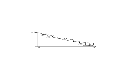
Figure 1: The Arrhenius cascade.

The potential $U(x)$ is a tilted random ’washboard’. It presents $n$ local minima or ’wells’, labelled by $i$, separated from the next minimum $i+1$ by a potential ’hill’ of random height $U_{i}$ (the $U_{i}$’s are independent variables). We assume an exponential probability density $f(U)$ for the hills $U_{i}$:

$$f(U)=\frac{1}{U_{0}}\;e^{-U/U_{0}}\,,$$ (3)

where $U_{0}$ is the average height of the potential hills. The variable $x$ may be a position coordinate or any coordinate of the system.

At any time, the physical system is trapped in one of the local potential wells. Due to thermal fluctuations, the system performs sudden jumps from one well to the other one downwards. The global tilt of the potential hill $U(x)$ is large enough to prevent the system from performing upward jumps. Therefore, the system can only cascade downwards. The trapping time $\tau_{i}$ in the well $i$ is related to $U_{i}$ by the Arrhenius law:

$$\tau_{i}=\tau_{0}\;e^{U_{i}/(k_{\rm B}T)}\,,$$ (4)

where $\tau_{0}$ is a characteristic time, $k_{\rm B}$ is the Boltzmann constant and $T$ is the temperature.

We consider a gedanken experiment in which the experimentalist wants to know the average trapping time in a single well, but can only measure the time $t_{n}$ needed to go through all the $n$ wells of the system:

$$t_{n}=\sum_{i=1}^{n}\tau_{i}\ \cdot$$ (5)

To reduce the measurement uncertainty, he can repeat $m$ times his measurement of $t_{n}$. We assume that, between each measurement, the realization of the disorder changes, i.e. the numbers $U_{1},...U_{n}$ change (and thus $\tau_{1},...\tau_{n}$ change accordingly). His estimation $\tau_{\rm exp}(N)$ of the average trapping time will therefore be:

$$\tau_{\rm exp}(N)=\frac{1}{N}\sum_{j=1}^{m}t_{n}=\frac{1}{N}\sum_{i=1}^{N}\tau_{i}\ ,$$ (6)

where $N=m\times n$ is the total number of explored wells and the $\tau_{i}$’s are independent random variables defined by Eq. (3) and (4).

2.2 Behaviour of the Arrhenius cascade

12cm

Figure 2: Simulated measurements of the estimated $\tau_{\rm exp}(N)$. We have chosen $n=10$ and $\tau_{0}=1$. The quantity $\tau_{\rm exp}(N)$ for the case $k_{\rm B}T=3U_{0}$ has been multiplied by 30 to be more visible.

Simulated measurements of $\tau_{\rm exp}(N)$ are represented in figure 2 for two different temperatures. For a temperature $T=3U_{0}/k_{\rm B}$, $\tau_{\rm exp}(N)$ converges nicely to the average value $\langle x\rangle$ when $N$ increases, after exhibiting reasonable fluctuations at small $N$. This is the expected, standard behaviour.

For a lower temperature $T=0.5U_{0}/k_{\rm B}$, the behaviour of $\tau_{\rm exp}(N)$ is markedly different. The measured $\tau_{\rm exp}(N)$’s do not seem to converge towards any constant value but rather to diverge in a very fluctuating way with increasing $N$. A detailed analysis would reveal that the $t_{n}$’s also fluctuate very much from one measurement to the other. This unusual statistical behaviour would puzzle most experimentalists: large fluctuations and irreproducibility are usually considered as the indication of a problem in the experimental procedure, arising from poorly controlled parameters. But here, one would find that the experimental setup works apparently well .

2.3 Application of the generalized CLT

Let us see how the generalized CLT can shed light on the previous observations. We first easily calculate the probability density $f(\tau)$ of the trapping times. It is given by the relation $f(\tau){\rm d}\tau=f(U){\rm d}U$, which leads immediately to

$$f(\tau)=\alpha\;\frac{\tau_{0}^{\alpha}}{\tau^{1+\alpha}}\quad{\rm with}\quad\alpha=\frac{k_{\rm B}T}{U_{0}}\;\cdot$$ (7)

Having a power law for $f(\tau)$, the probability densities of $\tau_{\rm exp}(N)$ at large $N$ are provided for any $\alpha$ by the generalized CLT.

In the high temperature case ($T=3U_{0}/k_{\rm B}$), we have $\alpha=3$ which is larger than 2. Thus $\langle\tau^{2}\rangle$ is finite and the usual CLT applies: $\tau_{\rm exp}(N)$ is gaussianly distributed at large $N$ and tends to $\langle\tau\rangle$. This agrees with the observations (figure 2) and does not need further discussion.

In the low temperature case ($T=0.5U_{0}/k_{\rm B}$), on the contrary, we have $\alpha=0.5$ which is smaller than 1. The usual CLT does not hold anymore and the specific features of the generalized CLT will play a crucial role. The generalized CLT tells us that we should consider the quantity $Z_{N}=\sum_{i=1}^{N}\tau_{i}/N^{1/\alpha}$ and that the density $f(Z_{N})$ tends to a Lévy law $L_{\alpha}(Z_{N})$ at large $N$. This theorem has several important physical consequences: scaling of the Lévy sums, domination of the Lévy sums by a single term and large fluctuations of the Lévy sums (most of these consequences are presented in [BoG90]). We only treat here the case $\alpha<1$ (and not $1\leq\alpha\leq 2$) for which the consequences of the generalized CLT depart most strongly from the ones of the usual CLT. These consequences are:

• The most probable value of the sum $T_{N}=\sum_{i=1}^{N}\tau_{i}$ scales as

  $$T_{N}\sim N^{1/\alpha}\,,$$ (8)

  and not as $N$ which is more usual. Practically, this implies that the time $t_{n}$ spent in an Arrhenius cascade of $n$ wells does not scale with the size $n$ of the cascade, but more rapidly due to the generalized CLT. Similarly, the experimental value $\tau_{\rm exp}(N)=\frac{1}{m\times n}\sum_{j=1}^{m}t_{n}$ does not tend to a constant for a large number of measurements $m$ but diverges with $m$, as $m^{-1+1/\alpha}$. This explains the observed behaviour in figure 2. Thus, the size of the system and the number of measurements play a non trivial role in the measured values, an unusual situation in physics.

• The notion of average value is irrelevant here since $\langle\tau\rangle=\infty$. One can somehow replace it by the notion of typical value, i.e. most probable value. When $\alpha<1$, the typical terms $x_{i}$ of a Lévy sum $X_{N}=\sum_{i=1}^{N}x_{i}$ are not all of the same order (as they are when $f(x)$ is a narrow density) but present a hierarchical structure. In particular, the typical largest term $x_{\rm max}$ of the sum can be shown to be of the same order of magnitude as the sum itself

  $$X_{N}=\sum_{i=1}^{N}x_{i}\simeq x_{\rm max}\,,$$ (9)

  however large $N$ might be (Eq. (9) is valid within prefactors that do not depend on $N$). This domination of a sum by a single term, or by a small number of terms, is a signature of Lévy statistics in a physical problem (see figure 3 below).

  It can be used cleverly in physical experiments as a ’Lévy microscope’: by measuring a macroscopic quantity $X_{N}=\sum_{i=1}^{N}x_{i}$, one may obtain an easy access to a microscopic information, $x_{\rm max}$, while the direct measurement of $x_{\rm max}$ (i.e. in the Arrhenius cascade, the direct study of a single well) can be physically impossible. Such advantageous use of the statistical domination of a single term has been made implicitly, for instance in studies of quantum tunneling [RoB84].

• A Lévy sum $X_{N}=\sum_{i=1}^{N}x_{i}$ fluctuates as much as a single term, when $\alpha<1$. This is a direct consequence of the domination of the sum by a single term. It can also be seen as a consequence of the fact that the tail of the Lévy law $L_{\alpha}(Z_{N})$, which determines the fluctuations, decays as $1/Z_{N}^{1/\alpha}$, exactly as the tail of $f(x)$. This explains the highly fluctuating $\tau_{\rm exp}(N)$ obtained in figure 2 as being intrinsically due to the type of involved statistics and not to some technical experimental problem. Thus, fluctuations do not vanish as usual with the increase of the size $N$ of the statistical sample. The sums $X_{N}$ retain an intrinsically large irreproducibility. This is in contradiction with a traditional motivation for applying statistical methods: to go beyond the irreproducibility of individual events in order to obtain quasi-perfect reproducibility for large ensembles of events. However, the generalized CLT still allows for some predictibility in the statistical sense, since it predicts the stable form of the probability density of $Z_{N}$.

  Physics has incorporated two new types of randomness during this century: quantum uncertainty and deterministic chaos. It seems to us that the non-averaging out of fluctuations in Lévy flights can also be recognized as an important type of randomness.

3 Subrecoil laser cooling of atomic gases

In the Arrhenius cascade (section 2), a sum of $N$ independent terms was directly measured and the generalized CLT could be applied directly to analyze the results. In this section, we proceed a step further by studying a richer physical problem, called subrecoil laser cooling. In this case, Lévy sums —and their properties dictated by the generalized CLT— play an essential role, although they are not measured directly.

We introduce subrecoil laser cooling in section 3.1. In section 3.2, we show that power law densities of time variables appear, which implies the non-ergodicity of the process. In section 3.3, the generalized CLT is used to get some insight on the cooling efficiency. In section 3.4, quantitative predictions are derived, using the ’sprinkling density’. In section 3.5, we indicate how the insight provided by the generalized CLT enables to optimize the cooling strategy.

The starting point of the approach presented here has been presented in [BBE94] and [Bar95]. A detailed description of the theory will appear in [BBA99].

3.1 Subrecoil laser cooling

Laser cooling of atomic gases is based on the momentum exchanges between photons and atoms. In standard (not subrecoil) laser cooling, laser configurations and atomic transitions are carefully chosen so that these momentum exchanges lead to a friction force. This friction force damps the thermal atomic momenta $p$, thereby reducing the momentum spread (standard deviation) $\delta p$ of the atomic gas, which is equivalent to reducing the effective temperature $T$ defined by

$$k_{\rm B}T=\delta p^{2}/M$$ (10)

where $k_{\rm B}$ is the Boltzmann constant and $M$ is the mass of the atoms. Temperatures commonly achieved in the last ten years are in the range of a few microkelvins, 8 orders of magnitude below room temperature. This has opened exciting new possibilities for atomic and quantum physics and has been a key ingredient in the realization, in 1995, of a new state of matter called Bose-Einstein condensate. The 1997 Nobel prize of physics was attributed to S. Chu, C. Cohen-Tannoudji and W. Phillips for their contributions to laser cooling.

Standard laser cooling mechanisms are fundamentally limited to temperatures larger than the so-called ’recoil temperature’. Indeed, among the momentum exchanges between atoms and photons, some —the ones due to spontaneous emission— occur in a random direction. Each spontaneous emission of a photon by an atom thus results in an uncontrollable random recoil of the atomic momentum $\vec{p}$ by a quantity $\hbar\vec{k}$, where $\hbar\vec{k}$ is the momentum of a single photon. Therefore, the standard deviation $\delta p$ of the atoms is expected to be always larger than $\hbar k$. This implies (cf. Eq. (10)) laser cooling temperatures $T$ larger than the recoil temperature defined by $T_{\rm R}=(\hbar k)^{2}/(k_{\rm B}M)$. The recoil temperature $T_{\rm R}$ is on the order of one microkelvin for the configurations frequently used.

To sum up, the randomness of spontaneous emission, which is essential for the cooling since it provides a dissipative contribution to the atomic evolution, is also harmful to the cooling since it implies a limit temperature. As spontaneous emission of photons by atoms placed in laser light seems unavoidable, the recoil temperature was for some time considered as an absolute limit for laser cooling.

Subrecoil laser cooling, i.e. $T<T_{\rm R}$, is however possible. Indeed, although spontaneous emission of photons is an intrinsically random quantum process, it can be partly controlled. The key idea is to create a spontaneous emission rate $R(p)$ which depends on the atomic momentum $p$ (figure 3) and which vanishes at $p=0$. This was first proposed and realised in 1988 [AAK88, AAK89] using a nice quantum effect called a ’dark resonance’, because a resonance occurs at $p=0$ which prevents the spontaneous emission. Today, record low temperatures reached experimentally with dark resonances approach $T_{\rm R}/1000$, which corresponds to a few nanokelvins only.

12cm

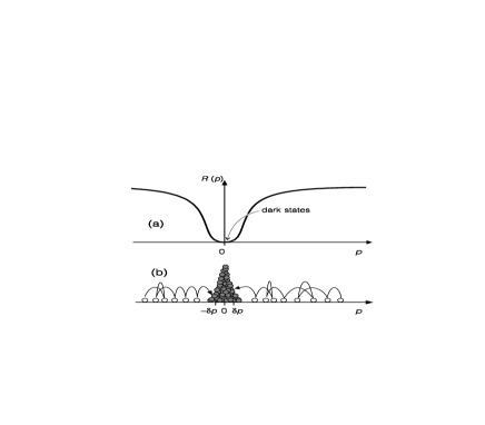
Figure 3: Principle of subrecoil cooling. a) The spontaneous emission rate $R(p)$ vanishes at momentum $p=0$. b) The atoms perform a momentum random walk and accumulate in the vicinity of $p=0$.

One can follow the evolution of an atom with an initially non-zero momentum $p$. The spontaneous emission rate $R(p)$ being large, the atom will spontaneously emit photons and therefore its momentum will change in a random way. This random walk will eventually lead by chance the atom in the vicinity of $p=0$ where the spontaneous emission rate is very small (see figure 3). There, the atom stops exchanging momentum with photons and it remains so-to-speak ’trapped’ in what is called a ’dark state’. The time $\tau(p)$ of residence at momentum $p$ is

$$\tau(p)=\frac{1}{R(p)}\ ,$$ (11)

the time interval between two spontaneous emissions. If this residence time is long enough, the atom keeps the same small momentum till the end of the experiment. If not, it emits a spontaneous photon, which starts a new momentum diffusion process and gives to the atom another chance to reach the vicinity of $p=0$. Thus atoms accumulate in the vicinity of $p=0$ in long-lived states: a cooling effect occurs. This cooling relies on a random walk of the atomic momentum, unlike standard laser cooling which rests on friction forces.

The most important question for a cooling process is to determine the typical momentum $\delta p$ at the end of the random walk or, equivalently the temperature $T$ (cf. Eq. (10)). It is difficult to answer it with the usual analytical or numerical methods of atomic physics because very different momentum and time scales are present in the problem. A conjecture was proposed in 1988 in which the interaction time $\theta$, defined as the time the atoms interact with the lasers, plays a crucial role. Consider an atom reaching a momentum $p$ such that the residence time $\tau(p)$ is larger than the interaction time $\theta$. This atom will thus keep its momentum $p$ till the end of the experiment and will be detected with this momentum $p$. The conjecture consists in assuming that only the atoms such that

$$\tau(p)\geq\theta$$ (12)

keep their momentum till the end of the experiment. Obviously, this can not be strictly true: some atoms will reach a small momentum $p$ after a significant time $t$ has elapsed from the beginning of the interaction with the lasers so that, for them, the condition to stay at momentum $p$ would rather be $\tau(p)\geq\theta-t$. But let us assume that condition (12) is the relevant criterion for the trapping of atoms. This predicts that a momentum peak will form with a width $\delta p_{\theta}$ given by

$$\tau(\delta p_{\theta})\simeq\theta\ \cdot$$ (13)

Moreover, it can be shown that the residence time $\tau(p)$ varies as

$$\tau(p)\propto 1/p^{2}\ \cdot$$ (14)

Introducing this relation into Eq. (13) gives the conjectured momentum scale $\delta p_{\theta}$ which is reached after an interaction time $\theta$:

$$\delta p_{\theta}\propto\frac{1}{\sqrt{\theta}}$$ (15)

or, for the temperature $T_{\theta}\propto(\delta p_{\theta})^{2}$ (cf. Eq. (10)),

$$T_{\theta}\propto\frac{1}{\theta}\;\cdot$$ (16)

This result is both interesting and surprising. Interestingly, it predicts that the temperature can be reduced towards lower and lower values when the interaction time $\theta$ is increased. The recoil temperature limit, which arises in standard laser cooling from spontaneous emission, is no more a limit here. Here indeed, spontaneous emission is present to create a random walk that brings the atoms to $p\simeq 0$, but spontaneous emission stops when the atoms reach a small enough momentum. Surprisingly, there does not seem to be any limit for the cooling.

This has motivated a series of experiments with longer and longer interaction times $\theta$. The recoil limit was first overcome in 1988, reaching $T_{\theta}\simeq T_{\rm R}/2$ [AAK88]. Longer interaction times allowed to reach $T_{\theta}\simeq T_{\rm R}/40$ in 1994 [BSL94, Bar95] and $T_{\theta}\simeq T_{\rm R}/800$ in 1997 [SHK97], establishing a new temperature record each time. Moreover, these experiments agree well with the conjectured temperature dependence of Eq. (16).

However, one obviously needs a better understanding of what determines the temperature $T_{\theta}$. A related question is the proportion of cooled atoms: can a random walk with no driving force lead to an accumulation of all the atoms in the vicinity of $p=0$? Is there rather only a small proportion of cooled atoms? How does this fraction vary with the interaction time $\theta$ and with the number of dimensions of the random walk? As we will see below, random walk techniques and the generalized CLT provide answers to these questions.

3.2 Trapping time densities and non-ergodicity

Recently developped quantum simulations [DCM92, DZR92, Car93, CBA91] allow to follow the momentum random walk of a single atom in the process of subrecoil cooling [CBA91, BBE94, Bar95]. An example of such a random walk is represented in figure 4. We see how the random evolution of the atomic momentum sometimes leads to $p\simeq 0$ states where the atom remains for a long time because the spontaneous emission rate $R(p)=1/\tau(p)$ vanishes in $p=0$: this is the principle of subrecoil cooling at work.

12cm

Figure 4: (a) Example of a momentum random walk resulting from a Monte-Carlo simulation of subrecoil cooling of metastable helium atoms. The unit of atomic momentum $p$ is the momentum $\hbar k$ of the photons. The zoom (b) of the beginning of the time evolution is statistically analogous to the evolution at large scale, a fractal property typical of a Lévy flight.

More importantly, figure 4 presents an interesting statistical feature that triggered the Lévy flight approach of laser cooling. The single largest residence time $\tau_{\rm max}$ amounts to 70 % of the total time $\theta$ while the atom has occupied 4000 different momentum states during this total time. Thus a single event dominates a sum of a large number of events, which is an indication of a Lévy flight.

Is there really a Lévy flight in the problem? Let us estimate the probability density $f(\tau)$ of trapping times $\tau$, defined as the times spent by an atom in an interval $[-p_{\rm trap};+p_{\rm trap}]$ called the ”trap” of size $p_{\rm trap}$ smaller than the size $\hbar k$ of a random momentum step. The probability density $\rho(p)$ for an atom reaching the trap to fall in a state of momentum $p$ can then be considered as independent of $p$ (in one dimension):

$$\rho(p)\simeq\frac{1}{2p_{\rm trap}}\;\cdot$$ (17)

The trapping time density $f(\tau)$, given by $f(\tau){\rm d}\tau=\rho(p){\rm d}p$, is easily obtained using Eq. (14):

$$f(\tau)\propto\frac{1}{\tau^{1+\alpha}}\quad{\rm with}\quad\alpha=\frac{1}{2}\;\cdot$$ (18)

Thus, if we consider as a first step that the interaction time $\theta$ is the sum of trapping times $\tau_{i}$ with the density (18), the time $\theta$ is indeed a Lévy sum, whose behaviour is dictated by the generalized CLT with $\alpha<1$. We have a Lévy flight in time, which immediately accounts for the domination of a single trapping event in figure 4 (see section 2.3).

There is a deep physical consequence of this Lévy flight, the absence of ergodicity. The ergodic hypothesis, an important ingredient in statistical physics, is the assumption that time averaging of a physical quantity yields the same result as ensemble averaging. Time averaging requires following a particle over a time much larger than all characteristic times of the problem. This is impossible here. Indeed, as the time $\theta$ gets larger, larger trapping time scales (up to $\theta$) appear and the time averaging procedure does not converge. This is reflected in the fact that we have a Lévy flight on a time variable $\tau$, with infinite average trapping times. Thus, subrecoil cooling is a non-ergodic process. The non-ergodicity is associated to the absence of cooling limits. The cooling goes on for ever because larger and larger trapping times $\tau(p)$, corresponding to lower and lower momenta $p$, can be reached with increasing $\theta$.

3.3 Trapping, recycling and the generalized CLT

The history of an atom over a time $\theta_{N}$ can be seen a series of $N$ trapping times $\tau_{i}$ interrupted by $N$ times $\hat{\tau}_{i}$ spent out of the trap. The times $\hat{\tau}_{i}$ are the usual ’first return times’. We also call them ’recycling times’ because the atoms coming out of the trap are given another opportunity to reach the trap, they are ’recycled’.

Thus, the interaction time $\theta_{N}$ writes as

$$\theta_{N}=\tau_{1}+\hat{\tau}_{1}+...+\tau_{N}+\hat{\tau}_{N}=T_{N}+\hat{T}_{N},$$ (19)

where

$$T_{N}=\sum_{i=1}^{N}\tau_{i}$$ (20)

is the total trapping time, and

$$\hat{T}_{N}=\sum_{i=1}^{N}\hat{\tau}_{i}$$ (21)

is the total recycling time. Both $T_{N}$ and $\hat{T}_{N}$ are sums of independent variables. The application of the generalized CLT to these sums gives in a simple way a qualitative answer for the proportion of cooled atoms, as we discuss now.

Consider first the case in which the spontaneous emission rate $R(p)$ tends to a non-vanishing constant at large $p$. Then, at large $p$, we have a standard random walk with a constant diffusion rate. For a 1D problem, the probability density $\hat{f}(\hat{\tau})$ of first return times $\hat{\tau}$ is known to decay at large $\hat{\tau}$ as

$$\hat{f}(\hat{\tau})\propto\frac{1}{\hat{\tau}^{1+\hat{\alpha}}}\quad{\rm with}\quad\hat{\alpha}=\frac{1}{2}\;\cdot$$ (22)

It thus decays exactly in the same way as $f(\tau)$. According to the generalized CLT, for large $N$’s, the sums $T_{N}$ and $\hat{T}_{N}$ behave as

$$T_{N} \sim N^{1/\alpha}=N^{2}\ ,$$ (23)

$$\hat{T}_{N} \sim N^{1/\hat{\alpha}}=N^{2}\,\cdot$$ (24)

Therefore, for long times (cf. large $N$’s), one has $T_{N}\sim\hat{T}_{N}$: the atoms spend a finite fraction of their time in the trap and a finite fraction outside the trap. We thus expect the proportion of cooled atoms to tend to a constant, strictly between 0 and 1. More elaborate calculations confirm this non-trivial result.

Consider now the case in which a friction mechanism is added to prevent the atoms to diffuse to too large momenta $p$. This friction confines the momentum diffusion in a finite zone. In this case, $\hat{f}(\hat{\tau})$ is a narrow probability density with a finite average value. Thus, according to the usual CLT:

$$\hat{T}_{N}\simeq N\langle\hat{\tau}\rangle\,\cdot$$ (25)

Comparing this to Eq. (23) which is still valid here, one has

$$T_{N}\gg\hat{T}_{N}$$ (26)

for large $N$. This implies that all the atoms will be cooled, which is again confirmed by more elaborate calculations.

More complicated cases can be considered by including diffusion in 2 or 3 dimensions or by including the ’Doppler effect’ which modifies the rate $R(p)$ at large $p$. In each case, the generalized CLT provides the asymptotic behaviours of the sums $T_{N}$ and $\hat{T}_{N}$ which yield immediately the qualitative asymptotic proportion of cooled atoms.

3.4 Momentum distribution

Up to now, we have presented mostly qualitative results. We want to sketch here how some quantitative results are obtained.

The main features of the cooling process are given by the momentum distribution (probability density) ${\mathcal{P}}(p,\theta)$ of trapped atoms at time $\theta$. This momentum distribution ${\mathcal{P}}(p,\theta)$ writes as an integral over the times $t_{l}$ at which the atoms enter the trap for the last time:

$${\mathcal{P}}(p,\theta)=\rho(p)\int_{0}^{\theta}{\rm d}t_{l}S_{\rm R}(t_{l})\psi(\theta-t_{l}|p)\;\cdot$$ (27)

The quantity $\rho(p)$ is the probability density for an atom entering the trap to reach the momentum $p$ (in one dimension, we have seen in Eq. (17) that $\rho(p)=1/(2p_{\rm trap})$). The quantity $S_{\rm R}(t)$ called here the ’sprinkling density’ is the probability density for an atom to return into the trap at time $t$, regardless of the number of times the atom has entered the trap before. The quantity $\psi(\tau|p)=\int_{\tau}^{\infty}f(\tau^{\prime}){\rm d}\tau^{\prime}$ is the probability that an atom remains in the trap during a time longer than $\tau$ (where $f(\tau)$ is the trapping time density defined in section 3.2).

The momentum distribution can be calculated explicitly. For instance, in a simple 1D model with infinite $\langle\tau\rangle$ and finite $\langle\hat{\tau}\rangle$, one obtains

$${\mathcal{P}}(p,\theta)=h(\theta){\mathcal{G}}(Ap\sqrt{\theta})$$ (28)

where $h(\theta)\propto\sqrt{\theta}$ is the height of the cooled peak at $p=0$, $A$ is a constant. The function ${\mathcal{G}}(q)$ is given by ${\mathcal{G}}(q)=1$ for $q\leq 1$ and by ${\mathcal{G}}(q)=1-(1-q^{-2})^{1/\alpha}$ for $q\geq 1$. The width $\delta p_{\theta}$ of ${\mathcal{P}}(p,\theta)$ decays as $1/\sqrt{\theta}$, which proves the 1988 conjecture of a temperature decrease without any fundamental limit (cf. Eq. (16)). This calculation can also be done for more complicated cases in any dimension where it is very useful. For instance, one can study the influence of the exponent $\beta$ in the spontaneous emission rate $R(p)\propto p^{\beta}$, as described in the next section.

The key point to obtain the momentum distribution is the calculation of the sprinkling density $S_{\rm R}(t)$. The sprinkling density is obtained relatively easily with a Laplace transform. The result is interesting. If $\langle\tau\rangle$ and $\langle\hat{\tau}\rangle$ are finite, then $S_{\rm R}(t)$ tends to a constant at large times. This is an expected ’ergodic’ result: the rate of return events is asymptotically constant. On the contrary, if $\langle\tau\rangle$ or $\langle\hat{\tau}\rangle$ is infinite, then $S_{\rm R}(t)$ decays to 0 at large times. This is a signature of non-ergodicity: at large times, the density of return events go to 0 because the longer and longer $\tau_{i}$’s or $\hat{\tau}_{i}$’s which tend to appear slow down the diffusion. Such a process has a ’history’: the measurement of $S_{\rm R}(t)$ at any time tells when the diffusion has started.

3.5 Optimizing laser cooling with the generalized CLT

A remarkable outcome of the usual CLT is that the statistical behaviour of Lévy sums $X_{N}$ at large $N$ is determined only by two parameters, $\langle x\rangle$ and $\langle x^{2}\rangle$. Thus, the detailed features of $f(x)$ can be forgotten if one is interested only in the large $N$ properties of the Lévy sums. Similarly, with the generalized CLT in the cases $\alpha\leq 2$, only the asymptotic power law behaviour of $f(x)$ is relevant to determine the behaviour of Lévy sums at large $N$. For a positive variable $x$, for instance, this power law is described by two parameters only, the exponent $\alpha$ and the prefactor of the power law. This can provide a useful insight when confronted to a complex physical phenomenon with many parameters: the generalized CLT shows that the many physical parameters combine into only two relevant statistical parameters.

Such an insight has been applied in practice to improve a subrecoil laser cooling mechanism called Raman cooling [KaC92]. Raman cooling, like the dark resonance cooling described in section 3.1, rests on a $p$-dependent spontaneous emission rate $R(p)$ analogous to the one in figure 3a. The main difference is that the rate $R(p)$ results from the superposition of pulses that can be chosen nearly arbitrarily. This gives flexibility to this mechanism and makes it a good case study for cooling optimization. On the other hand, the large number of parameters ($\simeq 30$ for the initially used sequence of pulses) to be optimized makes it necessary to find simplifying guidelines.

By carefully using the generalized CLT, we have proposed a new very simple sequence of pulses [RBB95]: it relies on 4 pulses only (compared to 14 initially); the shape of the pulses is the simplest possible while the initially used pulses were sophisticated Blackman pulses.

The results are eloquent. With the initially used sequence of 14 pulses, the temperature $T_{\theta}$ varied as $T_{\theta}\propto 1/\sqrt{\theta}$ with the interaction time $\theta$. With the new sequence of 4 pulses, the new shape (which changes the exponent $\beta$ of the rate $R(p)\simeq p^{\beta}$ from $\beta=4$ to $\beta=2$) leads to $T_{\theta}\propto 1/\theta$, a much faster cooling. Moreover, with this new shape, if the pulses parameters (width and position) are adapted to the considered interaction time $\theta$, one obtains an even faster cooling $T_{\theta}\propto 1/\theta^{4/3}$ [RBB95, Rei96].

These predictions have been successfully tested experimentally and led to record low temperatures ($2.8\pm 0.5$ nK) for a cesium gas. This shows how the generalized CLT can have significant practical consequences.

4 Imperfect Lévy flights

We have presented in sections 2 and 3 two examples where the generalized CLT applied perfectly. However, there are many physical cases where the generalized CLT is useful although the conditions to apply it are not, strictly speaking, mathematically fulfilled. This may occur either because the asymptotic decay of $f(x)$ is not purely a power law or because $f(x)$ is a truncated power law.

Let us first discuss the truncation problem, i.e. the cases in which $f(x)$ decays as $1/x^{1+\alpha}$ for $x<x_{0}$ and decays more rapidly for $x>x_{0}$ so that $\langle x\rangle$ and $\langle x^{2}\rangle$ are finite. In the mathematical sense, the usual CLT applies. However, due to the power law tail, the convergence to the asymptotic gaussian for the probability density of the Lévy sums can be extremely slow, being reached for $N$ typically of $10^{3}$ or larger [MaS94], while in most cases for which the usual CLT applies, the approximate convergence to a gaussian is obtained very rapidly, with typically $N\simeq 4-5$. As, in practice, one often deals with sums of a moderately large number $N$ of terms, the behaviour of the Lévy sums is often dictated by the Lévy laws for relevant $N$ values, while the gaussian behaviour is recovered only for irrelevantly large $N$ values.

Second, there are broad probability densities which decay only approximately as power laws. An example is provided by broad lognormal distributions, which have of course a finite second moment. They can be rewritten as power laws $1/x^{1+\alpha(x)}$ with a logarithmically varying exponent $\alpha(x)$. If the logarithmic part of $\alpha(x)$ is small enough, then the generalized CLT gives at least some qualitative guidelines for the behaviour of the Lévy sums. We have used such guidelines to study the tunneling of electrons through a thin layer of insulator, a problem which has both basic and applied interests. The striking finding related to the generalized CLT has been that the typical current density varies by more than 200 depending on the scale at which it is measured [Bar97, DBB98, DHB98] (see also [LaB93]), while the typical current density should be scale independent if there were no tails in the probability density of the current.

Acknowledgements

The Institut de Physique et de Chimie des Matériaux de Strasbourg is Unité Mixte de Recherches 7504 of Centre National de la Recherche Scientifique and of Université Louis Pasteur. The section 3 is mostly based on a long paper (to be published) in collaboration with J.P. Bouchaud (Saclay), A. Aspect (Orsay) and C. Cohen-Tannoudji (Paris). I also thank all the researchers with whom I collaborated on the quoted papers.

References

- [AAK88] A. Aspect, E. Arimondo, R. Kaiser, N. Vansteenkiste, and C. Cohen-Tannoudji, Laser Cooling below the One-Photon Recoil Energy by Velocity-Selective Coherent Population Trapping, Phys. Rev. Lett. 61, 826-829 (1988).
- [AAK89] A. Aspect, E. Arimondo, R. Kaiser, N. Vansteenkiste and C. Cohen-Tannoudji, Laser cooling below the one-photon recoil energy by velocity-selective coherent population trapping : theoretical analysis, J. Opt. Soc. Am. B 6, 2112-2124 (1989).
- [AlK96] V. A. Alekseev and D. D. Krylova, Fraction number of trapped atoms and velocity distribution function in sub-recoil laser cooling scheme, Optics Communications 124, 568-578 (1996).
- [Bar95] F. Bardou, Ph. D. Thesis, University of Paris XI Orsay, chapters IV and V (1995).
- [Bar97] F. Bardou, Rare events in quantum tunneling, Europhys. Lett. 39, 239-244 (1997).
- [BBA99] F. Bardou, J.-P. Bouchaud, A. Aspect, and C. Cohen-Tannoudji, Non-ergodic cooling: subrecoil laser cooling and Lévy statistics, to be published.
- [BBE94] F. Bardou, J.-P. Bouchaud, O. Emile, A. Aspect and C. Cohen-Tannoudji, Subrecoil Laser Cooling and Lévy Flights, Phys. Rev. Lett. 72, 203-206 (1994).
- [BoC97] M. Boguna and A. Corral, Long-Tailed Trapping Times and Lévy Flights in a Self-Organized Critical Granular System, Phys. Rev. Lett. 78, 4950-4953 (1997).
- [BoD95] J.P. Bouchaud and D.S. Dean, Aging in Parisi’s Tree, J. Phys. I (France) 5, (1995) 265-286.
- [BoG90] J.P. Bouchaud and A. Georges, Anomalous diffusion in disordered media: statistical mechanisms, models and physical applications, Phys. Rep. 195, 127-293 (1990).
- [BSL94] F. Bardou, B. Saubaméa, J. Lawall, K. Shimizu, O. Emile, C. Westbrook, A. Aspect and C. Cohen-Tannoudji, Sub-recoil laser cooling with precooled atoms, C. R. Acad. Sci. Paris 318, Série II, 877-885 (1994).
- [Car93] H. Carmichael, An Open Systems Approach to Quantum Optics, Springer-Verlag (1993).
- [CBA91] C. Cohen-Tannoudji, F. Bardou, and A. Aspect, Review of fundamental processes in laser cooling, Proceedings of Laser Spectroscopy X (Font-Romeu, 1991), edited by M. Ducloy, E. Giacobino, and G. Camy, 3-14 (World Scientific, Singapore, 1992).
- [DBB98] V. Da Costa, F. Bardou, C. Béal, Y. Henry, J.P. Bucher, and K. Ounadjela, Nanometric cartography of tunnel current in metal-oxide junctions, J. Appl. Phys. 83, 6703-6705 (1998).
- [DCM92] J. Dalibard, Y. Castin, and K. Mølmer, Wave-Function Approach to Dissipative Processes in Quantum Optics, Phys. Rev. Lett. 68, 580-583 (1992).
- [DHB98] V. Da Costa, Y. Henry, F. Bardou, and K. Ounadjela, Experimental evidence and consequences of rare events in quantum tunneling, submitted (1998).
- [DZR92] R. Dum, P. Zoller, abd R. Ritsch, Monte-Carlo simulation of the atomic master equation for spontaneous emission, Phys. Rev. A 45, 4879-4887 (1992).
- [KaC92] M. Kasevich and S. Chu, Laser Cooling below a Photon Recoil with Three-Level Atoms, Phys. Rev. Lett. 69, 1741-1744 (1992).
- [KSW97] H. Katori, S. Schlipf, and H. Walther, Anomalous Dynamics of a Single Ion in an Optical Lattice, Phys. Rev. Lett. 79, 2221-2224 (1997).
- [KSZ96] J. Klafter, M.F. Shlesinger and G. Zumofen, Beyond Brownian Motion, Physics Today 49, 33-39 (February 1996).
- [LaB93] F. Ladieu and J.P. Bouchaud, Conductance statistics in small GaAs:Si wires at low temperatures. I. Theoretical analysis: truncated quantum fluctuations in insulating wires, J. Phys. I (France) 3, 2311-2320 (1993).
- [MaS94] R.N. Mantegna and H.E. Stanley, Stochastic Process with Ultraslow Convergence to a Gaussian: The Truncated Lévy Flights, Phys. Rev. Lett. 73, 2946-2949 (1994). M.F. Stanley, Comment, Phys. Rev. Lett. 74, 4959 (1995).
- [MEZ96] S. Marksteiner, K. Ellinger, and P. Zoller, Anomalous diffusion and Lévy walks in optical lattices, Phys. Rev. A 53, 3409-3430 (1996).
- [OBL90] A. Ott, J.P. Bouchaud, D. Langevin, and W. Urbach, Anomalous Diffusion in ”Living Polymers”: a Genuine Lévy Flight?, Phys. Rev . Lett. 65, 2201-2204 (1990).
- [RBB95] J. Reichel, F. Bardou, M. Ben Dahan, E. Peik, S. Rand, C. Salomon and C. Cohen-Tannoudji, Raman Cooling of Cesium below 3 nK: New Approach Inspired by Lévy Flight Statistics, Phys. Rev. Lett. 75, 4575-4578 (1995).
- [Rei96] J. Reichel, PhD thesis, University of Paris VI (1996).
- [RoB84] C.T. Rogers and R.A. Buhrman, Composition of Noise in Metal-Insulator-Metal Tunnel Junctions, Phys. Rev. Lett. 53, 1272-1275 (1984).
- [SHK97] B. Saubaméa, T.W. Hijmans, S. Kulin, E. Rasel, E Peik, M. Leduc, and C. Cohen-Tannoudji, Direct measurement of the spatial correlation function of ultracold atoms, Phys. Rev. Lett. 79, 3146-3149 (1997).
- [Shl88] M.F. Shlesinger, Fractal time in condensed matter, Ann. Rev. Phys. Chem. 39, 269-290 (1988).
- [SWS93] T.H. Solomon, E.R. Weeks, and H.L. Swinney, Observation of Anomalous Diffusion and Lévy Flights in a Two-Dimensional Rotating Flow, Phys. Rev. Lett. 71, 3975-3978 (1993).
- [SZF95] M.F. Shlesinger, G.M. Zaslavsky, and U. Frisch (Eds), Lévy flights and related topics in physics, Springer-Verlag (Berlin), (1995).
- [SZK93] M.F. Shlesinger, G.M. Zaslavsky, and J. Klafter, Strange kinetics, Nature 363, 31-37 (1993).
- [SSY97] S. Schaufler, W. P. Schleich, and V. P. Yakovlev, Scaling and asymptotic laws in subrecoil laser cooling, Europhys. Lett. 39, 383-388 (1997).
- [TLS95] C. Tsallis, S.V.F. Lévy, A.M.C. Souza, and R. Maynard, Statistical-Mechanical Foundation of the Ubiquity of Lévy Distributions in Physics, Phys. Rev. Lett. 75, 3589-3593 (1995).
- [Tsa95] C. Tsallis, Non-extensive thermostatistics: brief review and comment, Physica A 221, 277-290 (1995).
- [Tsa97] C. Tsallis, Lévy distributions, Physics World, 42-45 (july 1997).
- [ZaA95] D.H. Zanette and P.A. Alemany, Thermodynamics of anomalous diffusion, Phys. Rev. Lett. 75, 366-369 (1995).
- [ZuK94] G. Zumofen and J. Klafter, Spectral random walk of a single molecule, Chem. Phys. Lett. 219, 303-309 (1994).