CLNS 00/1706

Novel Method of Measuring Electron Positron Colliding Beam Parameters

D. Cinabro, K. Korbiak

Department of Physics and Astronomy, Wayne State Univeristy,
Detroit, MI 48202, USA
R. Ehrlich, S. Henderson, N. Mistry

Laboratory of Nuclear Studies, Cornell Univeristy,
Ithaca, NY 14853, USA

(29 November 2000)

Abstract

Through the simultaneous measurement of the transverse size as a function of longitudinal position, and the longitudinal distribution of luminosity, we are able to measure the $\beta_{y}^{\ast}$ (vertical envelope function at the collision point), vertical emittance, and bunch length of colliding beams at the Cornell Electron-positron Storage Ring (CESR). This measurement is possible due to the significant “hourglass” effect at CESR and the excellent tracking resolution of the CLEO detector.

PACS numbers: 29.27.Fh, 41.75.Ht, 29.40

Submitted to Nuclear Instruments and Methods in Physics Research Section A: Accelerators, Spectrometers, Detectors and Associated Equipment

One of the difficult problems in colliding beam physics is the measurement of beam parameters at the collision point. In this letter, we present a method of making such a measurement using precision measurements of the luminous region with $e^{+}e^{-}\rightarrow\mu^{+}\mu^{-}$ events detected by a general purpose high energy physics experiment. Key to this measurement is the detailed geometry of the highly focused colliding beams, which leads to the “hourglass” effect.[1]

Tightly focused beams have a “waist” at the focal point of the final quadrupoles and their size grows away from this waist. The transverse beam size is given by

$$\sigma(z)=\sqrt{\epsilon\beta(z)}$$ (1)

where $\beta(z)$ is the amplitude or beta function, which depends on the longitudinal position, $z$, of the beam and the emittance, $\epsilon$, which is independent of $z$. Near a waist, $\beta(z)$ can be written as

$$\beta(z)=\beta^{\ast}+\frac{(z-z_{0{\rm beta}})^{2}}{\beta^{\ast}}$$ (2)

where $\beta^{\ast}$ is the value of the beta function at the waist and $z_{0{\rm beta}}$ is the longitudinal position of the waist. Thus the beam in the longitudinal and transverse dimensions forms an hourglass shape with a minimum size at $z_{0{\rm beta}}$.

The hourglass effect arises from the beam being in Gaussian shaped bunches with length $\sigma_{z}$. If the bunch length is long compared with the dimension of the waist, then little of the beam is colliding where the beam is narrowest. In this case, the longitudinal distribution of luminosity depends not only on $\sigma_{z}$, but also on the horizontal and vertical value of the beta function at the interaction point, $\beta^{\ast}_{x}$ and $\beta^{\ast}_{y}$, respectively. In addition if either $\beta^{\ast}$ is smaller than $\sigma_{z}$, luminosity does not improve as much as naively expected by making $\beta^{\ast}$ smaller.

The luminous region is defined by the overlap integral of two beams. Thus we expect the vertical width of the luminous region as a function of the longitudinal position to be given by

$$\sigma_{y}(z)=\sqrt{\frac{\epsilon_{y}}{2}\left(\beta_{y}^{\ast}+\frac{(z-z_{0{\rm beta}})^{2}}{\beta_{y}^{\ast}}\right)}\ ,$$ (3)

and similarly for the horizontal width. It is assumed that the emittances and $\beta^{\ast}$’s are the same for the two beams. The beam parameters for the Cornell Electron-positron Storage Ring (CESR) for the data discussed in this paper are given in Table 1.

Table 1: CESR beam parameters at zero bunch current during the time this measurement was made.

Parameter	Value ($\mu$m)
$\beta_{x}^{\ast}$	$1.1996\times 10^{6}$
$\epsilon_{x}$	0.21
$\beta_{y}^{\ast}$	17900
$\epsilon_{y}$	0.0010
$\sigma_{z}$	18100

All the parameters in Table 1 are given at zero bunch current. They are all expected to depend on the bunch current. We have previously observed that $\beta_{x}^{\ast}$ is reduced by roughly a factor of two in colliding beam conditions due to the dynamic beta effect.[2] Likewise, $\beta_{y}^{\ast}$ is expected to be reduced by about 25% due to beam-beam focusing. The vertical emittance depends on the beam-beam tuneshift parameter; for operation in the saturated tuneshift regime, the vertical beam size increases linearly with bunch current. Additionally, there are streak camera observations which show an increase in $\sigma_{z}$ as the bunch current increases.[3] The method described in this paper is aimed at measuring some of these dynamic effects by direct observation of the luminous region.

Note that these measurements are taken over a long time, about four months of CESR and CLEO running, and at many different machine conditions. Thus we expect only rough agreement with the parameters given in Table 1, but we should be sensitive to the dynamic effects discussed above. We expect to observe a larger $\epsilon_{y}$ and $\sigma_{z}$, and a smaller $\beta_{y}^{\ast}$ and $\beta_{x}^{\ast}$ than given in Table 1.

Figure 1 shows $\sigma_{y}$ as given by

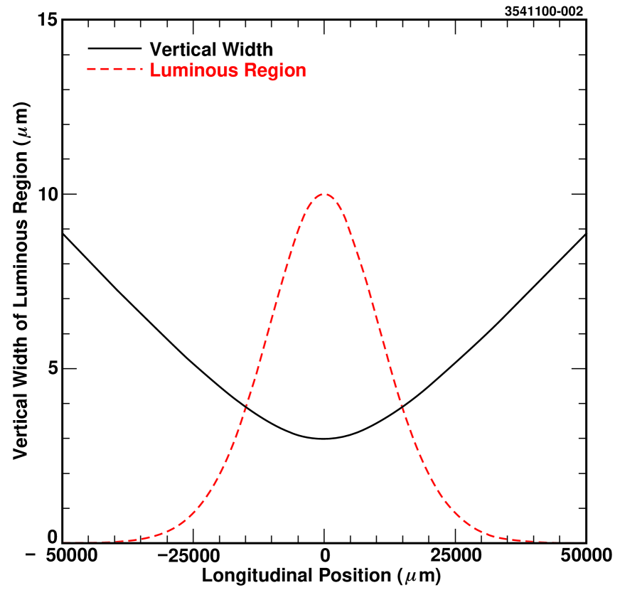
Figure 1: Expected vertical width of the luminous region as a function of longitudinal position. Also shown, in arbitrary units, is the expected longitudinal distribution of luminosity.

Equation 3 using the beam parameters given in Table 1. Also shown is the expected longitudinal distribution of luminosity. This is given by[1]

$$\frac{d{\cal L}}{dz}={\cal L}_{0}\frac{\exp{\left(\frac{-(z-z_{0{\rm bunch}})^{2}}{\sigma_{z}^{2}}\right)}}{(1+\frac{(z-z_{0{\rm beta}})^{2}}{\beta_{x}^{\ast 2}})^{1/2}(1+\frac{(z-z_{0{\rm beta}})^{2}}{\beta_{y}^{\ast 2}})^{1/2}}\ ,$$ (4)

where $z_{0{\rm bunch}}$ is the longitudinal position of the bunch-bunch collision. Note the longitudinal distribution of luminosity is expected to significantly depend on $\beta_{y}^{\ast}$, but the $\beta_{x}^{\ast}$ dependence is negligible. This is due to the large size of $\beta_{x}^{\ast}$ as compared to $\sigma_{z}$. Thus we expect a negligible hourglass effect in the horizontal size of the luminous region as a function of longitudinal position. This is also why we consider only one value for $z_{0{\rm beta}}$ which could, in principle, be different for the horizontal and vertical beta functions.

Our goal is to measure the beam parameters, $\beta_{y}^{\ast}$, $\epsilon_{y}$, and incidentally $\sigma_{z}$. We do this with a simultaneous fit to the measured vertical width of the luminous region versus longitudinal position, and the longitudinal distribution of luminosity. The vertical width depends on $\epsilon_{y}$, the longitudinal distribution on $\sigma_{z}$ and they both depend on $\beta_{y}^{\ast}$.

CESR has been described in detail elsewhere. [4] All the data used in this measurement are taken at an $e^{+}e^{-}$ collision energy of 10.58 GeV, and with bunch currents in the range of 2.5 to 7.0 mA over a four month period in late 1998 and early 1999. The CLEO detector has also been described in detail elsewhere.[5] All of the data used in this measurement are taken in the CLEO II.V configuration which includes a silicon strip vertex detector which is crucial to the measurement of the luminous region. This consists of three layers of silicon wafers arrayed in an octagonal geometry around the interaction point. The first measurement layer is at a radius of 2.3 cm and the wafers are read out on both sides by strips which are perpendicular to each other. The readout strips have a pitch of about 100$\ \mu$m and with charge sharing the detector has an intrinsic per point resolution of better than 20$\ \mu$m in both the transverse plane and the longitudinal direction

To obtain a resolution of order 10$\ \mu$m on the luminous region, we selected $e^{+}e^{-}\rightarrow\mu^{+}\mu^{-}$ events. These are easily selected in CLEO as events with two and only two tracks each with momentum near the beam energy and a small energy deposit in the electromagnetic calorimeter. We chose tracks with 20 or more hits in the main drift chamber, and at least two silicon vertex detector hits in the transverse and longitudinal views. We require that the tracks have opposite charge and that those used for the measurement of the luminous region have at least three silicon vertex detector hits in one of the two views.

We implement a method, called the “box technique,” to obtain measurements of the beam parameters and the resolution. Figure 2

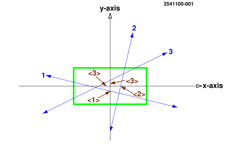
Figure 2: An ensemble of stiff tracks passing through the box allows for a precision measurement of the luminous region. For example, the track labeled 1 only gives a useful measure of the vertical position of the luminous region, as indicated. Track 1 crosses the the entire horizontal extent of the box and its average horizontal position is simply the center of the box, rather than the center of the luminous region. Similarly track 2 only measures the horizontal position, while track 3 measures both the horizontal and vertical positions of the luminous region.

shows how this technique is implemented. First, the size and location of the luminous region are obtained from run average data using hadronic events.[2] A three-dimensional box is then centered about the measured center of the luminous region with sides ten times the measured widths of the luminous region. The average position of a track passing through the box is found. From an ensemble of such positions the size and shape of the luminous region is measured.

Tracks that are parallel to an axis of interest are the most useful for measuring the luminous region. Tracks that are perpendicular to an axis cross the full length of the box in that direction and give no information about the luminous region. We select appropriate tracks by cutting on the direction cosines. Essentially, these cuts are determined by the size of the luminous region, which is roughly 10 $\mu$m vertically, 300 $\mu$m horizontally, and 10000 $\mu$m longitudinally. Thus a tight cut of $|p_{y}/p|\equiv|\cos\theta_{y}|<0.1$ is needed to measure the vertical luminous region, a looser cut of $|\cos\theta_{x}|<0.3$ for horizontal, and $|\cos\theta_{z}|<0.7$ for longitudinal. For tracks with large $|\cos\theta_{z}|$, the resolution degrades, and the $|\cos\theta_{z}|$ cut of $0.7$ is also used on tracks to make vertical and horizontal measures. Because of these direction cosine cuts, a single track can measure, at most, two dimensions.

We tested this method using over 100,000 $e^{+}e^{-}\rightarrow\mu^{+}\mu^{-}$ simulated events. To measure the change in the vertical size of the luminous region as expected from the hourglass effect, a constant vertical resolution is necessary. Thus we made selections in the simulated data to test the stability of the resolution and found significant dependences only on tracks with large values of $|\cos\theta_{z}|$, which are eliminated by the direction cosine cut discussed above, and on the $|\cos\theta_{y}|$ of the tracks. The $0.1$ cut on the $|\cos\theta_{y}|$ is a compromise between a smaller cut value with improved resolution, and a larger value with increased statistics. Thus the resolution on the vertical luminous region is expected to be $26.4\pm 0.4\pm 1.5\ \mu$m with the first error due to the statistics of the simulation sample and the second due to the sharp dependence on the $|\cos\theta_{y}|$ cut. This vertical resolution is small enough and there are sufficient data to obtain a statistically useful sample to measure the size of the luminous region at large longitudinal positions. These can be compared with similar measures dominated by the resolution taken at small longitudinal positions. In the analysis, we extract the resolution from the data itself, thus there is no dependence on the prediction from the simulation.

Figure 3 shows the vertical width of the luminous region as a function of its longitudinal position.

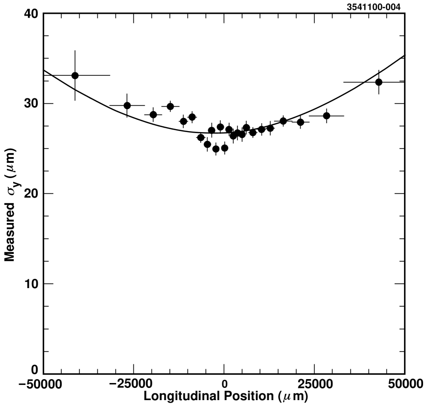
Figure 3: The vertical width of the luminous region as a function of longitudinal position. The line shows the fit discussed in the text.

This plot clearly shows the vertical distribution growing away from the center. This is evidence of the hourglass effect. We have also repeated this procedure for the horizontal width. We observe a horizontal width of 296 $\mu$m and see no significant hourglass effect. These observation both agree with our expectation.

When measuring the longitudinal distribution of luminosity as a function of the longitudinal position, we see a sharp enhancement in the distribution for small values of the longitudinal position. This enhancement is caused by the existence of a non-sensitive region in the center of the detector which greatly diminishes the chance for tracks passing through this region to be accepted for analysis. This geometric effect is accurately modeled in our simulation, and we use it to extract a longitudinal position dependent correction for the longitudinal distribution of luminosity. Applying this efficiency eliminates large systematic effects in our extraction of $\beta_{y}^{\ast}$. The longitudinal distribution of luminosity both before and after the efficiency correction is shown in Figure 4.

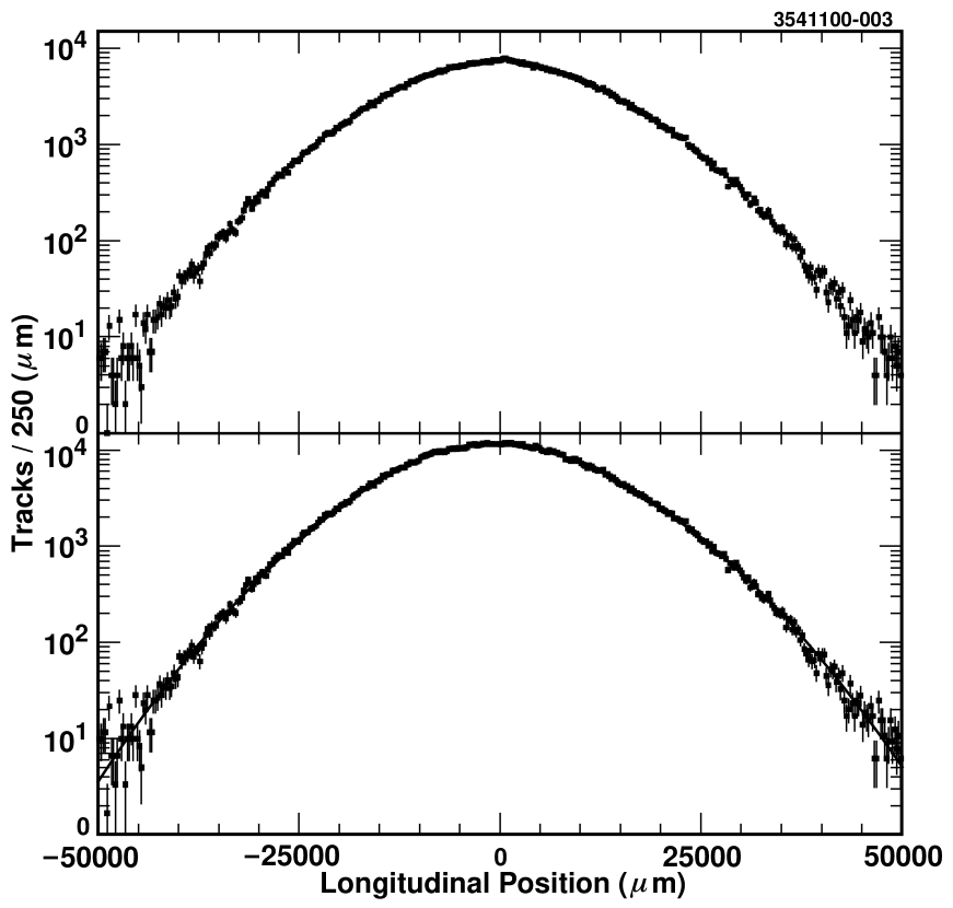
Figure 4: The longitudinal distribution of luminosity. The top plot shows the raw distribution. Note the slight enhancement near zero caused by detector geometry as discussed in the text. The bottom plot shows the efficiency corrected distribution with the fit discussed in the text superimposed.

To extract the beam parameters, we fit Figure 3 to Equation 3, including resolution smearing. Unfortunately, such a fit does not give a useful measurement of any of the beam parameters, and has nearly 100% correlations among $\beta_{y}^{\ast}$, $\epsilon_{y}$, and the resolution. We take advantage of the dependence of the longitudinal distribution of luminosity on $\beta_{y}^{\ast}$ as given in Equation 4, and perform a simultaneous maximum likelihood fit to Figures 3 and 4 to Equations 3 and 4. This simultaneous fit gives us an additional constraint on $\beta_{y}^{\ast}$ which breaks the correlations among the parameters.

In this fit we fix the value of $\beta_{x}^{\ast}$ to 417500 $\mu$m based on our observation of the horizontal width of the luminous region and the expected $\epsilon_{x}$ given in Table 1. The results are not sensitive to the exact value of $\beta_{x}^{\ast}$ used in the fit and change negligibly if $\beta_{x}^{\ast}$ is left to float. If $\beta_{x}^{\ast}$ is left to float the fit returns a value consistent with 417500 $\mu$m but with large errors of $\pm$500000 $\mu$m.

The resolution of the box technique on the longitudinal position of the event production point is better than $40\ \mu$m. This is negligible in comparison with the longitudinal size of the luminous region, which is over one centimeter. In fact, the box technique can be used to make a very high precision measurement of the bunch length, $\sigma_{z}$. As discussed in Reference [3] the bunch length in CESR is seen to depend on the bunch current and the bunches are asymmetric with their heads being narrower than their tails. Due to the collision of the two bunches this single bunch asymmetry is washed out in the longitudinal distribution of the luminous region. The luminosity distribution would only be distorted away from a Gaussian shape if the single bunch asymmetry were an order of magnitude larger than the observed $\sim 5$%. If we allow an asymmetry in the luminosity distribution, we observe none with a $\pm 1$% accuracy. This also confirms our need for an efficiency correction which takes out a $1.5$% asymmetry in the raw data.

We have tested this simultaneous fit procedure with the simulation, and expect that our fit is able to measure the input beam parameters and the resolution. We also derived expectations on the errors and correlations the fit should return based on our data statistics.

Table 2 shows the results of the fit to the data.

Table 2: The results of the simultaneous fit to the data distributions for the vertical width of the luminous region as function of longitudinal position and the longitudinal distribution. Only statistical errors are shown.

Parameter	Fitted Value ($\mu$m)
$\beta^{\ast}_{y}$	$15699\pm 138$
$\epsilon_{y}$	$0.0060+0.0047-0.0042$
$\sigma_{z}$	$19288\pm 38$
resolution	$25.8\pm 1.7$
$z_{0{\rm beta}}$	$-2885\pm 101$
$z_{0{\rm bunch}}$	$852.8\pm 34.7$

From the fit we observe some large correlations. These are between $\beta_{y}^{\ast}$ and $\sigma_{z}$, between $\epsilon_{y}$ and the resolution, and between $z_{0{\rm beta}}$ and $z_{0{\rm bunch}}$ These correlations are -88%, -75%, and -85% respectively. They are of the size predicted by our tests on simulated data. All other correlations are smaller than 40% in magnitude..

These are in good agreement with the errors expected from the simulation study, the CESR beam parameters of Table 1, and streak camera observations.[3] Note that we obtain very accurate measures of $\beta_{y}^{\ast}$ and $\sigma_{z}$, along with a resolution from the data consistent with our expectation of $26.4\pm 1.6\ \mu$m from the simulation, but only a 1.4 standard deviation measure of $\epsilon_{y}$. The results follow our expectations from the dynamic effects caused by the non-zero bunch current. The value for $\beta^{\ast}_{y}$ is lower than the zero bunch current value, but not as small as the lowest recorded. The value for $\epsilon_{y}$ is not measured well enough to make a meaningful test, but it is certainly consistent with an increase. The $\sigma_{z}$ is increased by 6.6% which is consistent with the streak camera observations.[3] The difference between $z_{0{\rm beta}}$ and $z_{0{\rm bunch}}$, $-3740\pm 130\ \mu$m, is consistent with known strength differences between the final focus quadrupoles and alignment tolerances between final focus elements and RF cavities which respectively determine the longitudinal position of the beta waist and the center of the bunch collision.

In an attempt to improve the measure of $\epsilon_{y}$, we repeat the data fit with the resolution fixed to $26.4\ \mu$m, as predicted by the simulation. This fit does give a slightly improved measurement of $\epsilon_{y}$ of $0.0049\pm 0.0028\ \mu$m with the other parameters changing negligibly. When we vary the fixed resolution by $\pm 1.6\ \mu$m as indicated by the simulation studies, this introduces an error of $\pm 0.0028\ \mu$m on $\epsilon_{y}$. The combined error of $\pm 0.0040\ \mu$m on $\epsilon_{y}=0.0049\ \mu$m is consistent with, but not a substantial improvement over the results of Table 2. We prefer to quote results for the fit where the resolution is left floating.

We varied the standard fit to test its robustness. We excluded positive $z$, negative $z$, small $z$, and large $z$ data from the fit. A $\chi^{2}$ fit is used rather than a likelihood fit. The only parameters that show significant disagreement with the standard result are $\beta_{y}^{\ast}$ and $\sigma_{z}$. Other facets of the analysis are varied and the procedure is repeated to estimate other systematic effects. Cuts on the direction cosines are varied, $\pm 0.01$ on $\cos\theta_{y}$ and $\pm 0.1$ on $\cos\theta_{z}$, we relax the three silicon vertex detector hits in one view to a looser two hit per view requirement, we vary the procedure for applying the efficiency for the luminosity as a function on the longitudinal position, and use the simulation efficiency without errors as an estimate of the effects of our limited simulation statistics. Some of the measured vertical widths are not consistent with their longitudinal neighbors as can be seen in Figure 3. This indicates a systematic error of about two microns in the extraction of the widths with the box method. Including this error has a negligible impact on the results of the fit, increasing the statistical errors by less than 10%. For all these variations, the change in the central values of the beam parameters from the standard procedure is taken as the systematic effect. The combined effects of these variations result in a systematic error of $\pm 460\ \mu$m on $\beta_{y}^{\ast}$, $\pm 0.0019\ \mu$m on $\epsilon_{y}$ and $\pm 200\ \mu$m on $\sigma_{z}$.

In conclusion, we use a new box technique to measure the size of the luminous region of CESR at the CLEO interaction region. This new method takes advantage of the hit resolution in the CLEO II.V silicon vertex detector and the well understood CLEO charged particle tracking system in $e^{+}e^{-}\to\mu^{+}\mu^{-}$ events to precisely measure the size of the luminous region. The technique has a resolution of $25.5\pm 2.0\ \mu$m which we extract from a fit to the data. The excellent resolution of the box technique, combined with the large size of the CLEO II.V data set, allows us to make a clear observation of the hourglass effect, the increase in the size of the luminous region away from the focal point. The technique leads to measurement of the CESR beam parameters:

$$\beta_{y}^{\ast} = (15700\pm 140\pm 460)\ \mu{\rm m},$$ (5)

$$\epsilon_{y} = (0.0060\pm 0.0045\pm 0.0019)\ \mu{\rm m},$$ (6)

$$\sigma_{z} = (19290\pm 40\pm 200)\ \mu{\rm m}.$$ (7)

where the first error is statistical and the second is systematic, in a simultaneous fit of the vertical width of the luminous region as a function of the longitudinal position and of the longitudinal distribution of the luminosity. Note that these measurements imply that the vertical width of the CESR beam at the CLEO collision point is $6.9\pm 2.8\ \mu$m. These measurement are in good agreement with the expectations of the theoretical CESR lattice taking into account the dynamic effects caused by the non-zero bunch current. This technique provides a non-invasive way to measure beam parameters at the collision point, but it requires the comparatively rare $e^{+}e^{-}\to\mu^{+}\mu^{-}$ events and a well understood detector tracking system.

References

- [1] D. Rice private communication; S. Milton, Cornell Colliding Beam Note 89-1 (unpublished); M. A. Furman, Proceedings Particle Accelerator Conference 1991, 422.
- [2] D. Cinabro, et al Physical Review E57, 1193 (1998).
- [3] R. Holtzapple, et al, Phys. Rev. ST Accel. Beams 3, 034401.
- [4] S.B. Peck and D.L. Rubin, ”CESR Performance and Upgrade Status,” Proceedings Particle Accelerator Conference 1999, 285.
- [5] Y. Kubota, et al. (CLEO Collaboration), Nuclear Instruments and Methods, A820, 66 (1990); T.S. Hill, Nuclear Instruments and Methods in Physics Research, A418, 32, (1998).