Modelling Horizontal and Vertical Concentration Profiles of Ozone and Oxides of Nitrogen within High-Latitude Urban Areas

Abstract

Urban ozone concentrations are determined by the balance between ozone destruction, chemical production and supply through advection and turbulent down-mixing from higher levels. At high latitudes, low levels of solar insolation and high horizontal advection speeds reduce photochemical production and the spatial ozone concentration patterns are largely determined by the reaction of ozone with nitric oxide and dry deposition to the surface. A Lagrangian column model has been developed to simulate the mean (monthly and annual) three-dimensional structure in ozone and nitrogen oxides ($NO_{x}$) concentrations in the boundary-layer within and immediately around an urban areas. The short time-scale photochemical processes of ozone and $NO_{x}$, as well as emissions and deposition to the ground, are simulated.

The model has a horizontal resolution of 1x1km and high resolution in the vertical. It has been applied over a 100x100km domain containing the city of Edinburgh (at latitude $56^{\circ}$N) to simulate the city-scale processes of pollutants. Results are presented, using averaged wind-flow frequencies and appropriate stability conditions, to show the extent of the depletion of ozone by city emmisions. The long-term average spatial patterns in the surface ozone and $NOx$ concentrations over the model domain are reproduced quantitatively. The model shows the average surface ozone concentrations in the urban area to be lower than the surrounding rural areas by typically $50\%$ and that the areas experiencing a $20\%$ ozone depletion are generally restricted to within the urban area. The depletion of the ozone concentration to less than $50\%$ of the rural surface values extends only 20m vertically above the urban area. A series of monitoring sites for ozone, nitric oxide and nitrogen dioxide on a north-south transect through the city - from an urban, through a semi-rural, to a remote rural location - allows the comparison of modelled with observed data for the mean diurnal cycle of ozone concentrations. In the city-centre, the cycle is well reproduced, but the ozone concentration is consistently overestimated.

Key-word index: Tropospheric ozone, Lagrangian column model, urban, nitrogen oxides, vertical exchange.

1 Introduction

Tropospheric ozone is a photochemical oxidant formed largely by photochemical reactions. In the troposphere ozone acts as a greenhouse gas (?), (?) and is toxic to plants, reducing crop yields (?), and to humans as a respiratory irritant (?), as well as damaging both natural and man-made materials, such as stone, brick-work and rubber, (?). Quantifying the dose and exposure of the human population, vegetation and materials to ozone is required to assess the scale of ozone impacts and to develop control strategies.

A network of 17 rural ozone monitoring stations across the UK provides broad-scale regional spatial patterns in tropospheric ozone concentrations in rural areas (?). Peak ozone concentrations increase from north to south across the UK as the south has higher concentrations of the primary pollutants necessary for ozone production (from greater emissions and proximity to continental sources) as well as greater frequency of meteorological conditions suitable for ozone production. Mean ozone concentrations also increase with altitude (?) and are higher in a 5-10km coastal strip (?). The mean annual-average background concentration of ozone for the UK is approximately 50$\mu$g m^-3, though there is a wide variation for individual episodes about this value, ranging up to about 400$\mu$g m^-3 (?). There are clear diurnal and annual cycles in ozone concentrations in the UK, with a mid-afternoon peak and nocturnal minimum and a spring maximum and autumn minimum. The diurnal cycle illustrates the fundamental importance of vertical mixing (?).

Ozone concentrations in urban areas are of particular interest and importance as the population is largely urban-based and ozone concentrations show greater spatial and temporal variations in urban areas. Ozone concentrations are smaller in urban areas than they are in surrounding rural areas due to the reaction of ozone with nitric oxide, emitted from combustion sources, forming nitrogen dioxide. Where air is allowed to stagnate over an urban area, the effects of strong insolation and accumulating ozone precursors can produce very high ozone concentrations. An example of this is the photochemical smog that affects the Los Angeles area of California, where a combination of meteorology, local topography and very high pollutant emission levels produce dangerously high ozone concentrations on many days of the year (?). However, in much of the UK and other high-latitude areas where insolation levels are lower and wind-speeds are larger (maintaining a steady advection of air through the urban air-shed), there is a different spatial distribution of concentrations with annual mean ozone concentrations generally smaller in urban areas.

There are many urban sites at which ozone is monitored in the UK (?). Attempts to map ozone concentrations using both rural and urban monitoring are complicated by the interaction of local chemistry with the larger-scale meteorological factors determining ozone concentrations. Recent studies on higher resolution ozone mapping have used an urbanisation index (?), but these have not been able to account for the movement of ozone and ozone-depleted air into and out of the urban areas.

Various studies have examined the characteristics of ozone and nitrogen oxide concentrations around urban areas (?). A large number of studies have focussed on the two-dimensional structure of the ‘urban plume’ of photochemical-ozone downwind of a city, with different cities around the world being studied (?), (?), (?), (?) and (?). There have been few studies of the three-dimensional mean structure of ozone concentrations in urban areas, especially at high latitudes, where ozone production is of secondary importance in describing the spatial distributions around cities. These studies are largely interpretations of observational data (?) and (?).

A boundary-layer Lagrangian column model has been developed to simulate the mean three-dimensional structure in ozone and nitrogen oxide concentrations in the boundary-layer within and immediately around high-latitude urban areas at a spatial scale of 1x1km. (The model is not appropriate for use with “real time” trajectories.) The model simulates the effects of ozone depletion at the surface as a consequence of the reaction with emitted nitric oxide and dry deposition to the surface. This has been used to follow a range of one-dimensional trajectories over a distance of $10^{5}$m and a travel time in the order of $10^{4}$s, through a simulated city under a variety of meteorological and pollutant emission regimes representing seasonal and diurnal extremes. An assessment of the extent of ozone destruction occurring, the rate of recovery of surface ozone concentrations downwind of the city and the influence of meteorological parameters on the ozone concentration has been provided using the model.

The model has been applied over a 100x100km domain containing a simulation of the emission field over the city of Edinburgh. Edinburgh was used as a generic, high-latitude city for modelling purposes. A land-use array has been created as input to the model with spatially- and temporally-variable emission and deposition values.

2 Ozone Destruction by Nitric Oxide

High latitude cities are, in general, well-ventillated, so that the timescale for air traversing the city is small compared to that for ozone generation. Under these conditions, the three reactions that are fundamental in the determination of ozone ($O_{3}$) concentrations in urban areas (?) are:

$$O+O_{2}+M\rightarrow O_{3}+M\hskip 51.21504ptk_{1}$$ (1)

$$NO_{2}+\it{h\nu}\rightarrow NO+O\hskip 51.21504ptJ_{2}$$ (2)

$$NO+O_{3}\rightarrow NO_{2}+O_{2}\hskip 51.21504ptk_{3}$$ (3)

where $k_{1}$ and $k_{3}$ are reaction rate constants and $J_{2}$ is the photolysis rate for nitrogen dioxide ($NO_{2}$).

In the UK, the main source of nitrogen oxides is the combustion of fossil fuels, $\it{ie.}$ the burning of coal, oil and gas in power stations and the combustion of petrol and diesel by road traffic (?). The largest source in large urban areas is the exhaust from road vehicles. The emissions are mainly $NO$ with ratios of $NO$:$NO_{2}$ in excess of about 3:1 (?). A large amount of this $NO$ is rapidly oxidised by ozone (Reaction 3).

The diurnal cycle of urban ozone concentrations show a maximum concentration at night from 0100 to 0500 hours when traffic density, and hence $NO$ emissions, are lowest (?). Minimum concentrations occur when the $NO$ concentration peaks during the morning and evening rush hours. Wind-speed also has an effect on urban ozone concentrations with ozone-rich air advected into the city from the surrounding countryside in windy condition. At the same time, $NO$ emitted in the city is diluted in the well-mixed air and so Reaction (3) is less dominant - reducing both $O_{3}$ destruction and $NO_{2}$ production (?).

3 Experimental Method

3.1 Description of the Model Used

The TERN model (Transport over Europe of Reduced Nitrogen) was developed in the early 1990s (?) to examine the release, transport and chemistry of ammonia. It is a Lagrangian column model with detailed vertical resolution and diurnally varying emissions, deposition and turbulent mixing. It was further developed to examine ammonia and ammonium transport and deposition over the UK (?). It can be used to obtain vertical concentration profiles of pollutants emitted or generated at or near the surface and transported over long distances on a single trajectory.

This Lagrangian column model was considered suitable as a basis for a model to be used in this study of urban ozone concentrations because it allows detailed vertical mixing to be considered and thus is able to represent the marked variations with height of the concentration profiles. An Eulerian model with a comparable run-time would not give the required vertical resolution (?). The TERN model has been considerably modified so as to be more suitable to modelling ozone concentrations in a city but the basic processes of calculating the extent of vertical mixing and the exchange between the vertical layers have remained the same. The detailed vertical resolution was used to provide a sophisticated treatment of the vertical diffusion of the pollutant species. The column of air that is advected over the surface (in the absence of vertical shear in the column) is the lowest 2.5km of the troposphere and is divided into 33 layers. There is much finer resolution near the surface (the lowest five layers are of depth 1, 2, 2, 4 and 15m), allowing more detail where the highest concentration gradients occur. The neglect of lateral dispersion, both by shear and turbulence, is not a serious omission for two reasons: firstly, the model is principally used to determine mean fields, for which climatological wind data are used, covering the whole 360 degrees; and secondly, the relatively small spatial scale of both the application of the model (and the resulting fields), means that changes due to lateral mixing are small compared to those due to vertical mixing.

Parameterisation of the boundary layer includes the effects on the mixing layer depth and the vertical diffusivity of the meteorological variables - insolation, cloud cover and wind-speed. The mixing layer depth is calculated on a diurnally varying pattern depending on the time of day and the prevailing meteorological conditions. Carson’s model (?) is used to calculate the development during the day, with a mechanical mixing factor proportional to the geostrophic wind-speed. At night, the depth is determined from a combination of the Pasquill category and the wind-speed (?).

The vertical mixing of gases, is determined using the diffusion equation:

$$\frac{\delta C}{\delta t}=\frac{\delta}{\delta z}\left(K_{z}\frac{\delta C}{\delta z}\right)$$ (4)

The coefficient of mixing, $K_{z}$, is defined as a function of height for different stability conditions. In the model, $K_{z}$ is assumed to linearly increase with height to a value of $K_{max}$ at height $z_{m}$ and to be constant above this height up to the top of the mixed layer. During the day, $z_{m}$ is fixed at 200m and $K_{max}$ is dependent on the larger of two terms, one representing mechanical mixing and the second on convective mixing. The first of these terms is dependent on stability and wind speed and the second on surface heat flux. At night, both $K_{max}$ and $z_{m}$ are dependent on wind speed and cloud cover (?).

TERN’s treatment of mechanical turbulence takes no account of the surface roughness. However, in the city the increased roughness effect of the buildings would increase the turbulence of the air compared to the countryside. Assuming a logarithmic wind profile over the lowest 200m (with no zero-plane displacement) and surface roughnesses of 0.05m for rural and 1.0m for urban areas (?), the ratio of urban to rural friction velocities was calculated to be 1.5. This factor is used as a scaling factor for $K_{z}$ to simulate enhanced mixing over urban areas.

A diurnally-varying dry deposition velocity ($V_{D}$), is included for nitrogen dioxide and ozone (?).

The chemistry employed in the model is very simple, with ozone destruction and production by Reactions (1-3) included but ozone production through hydrocarbon degradation ignored. Photodissociation (Reaction 2) is dependent on radiation levels which are parameterised in terms of time of day, time of year and climatological cloud cover.

The time-step used can be varied over a wide range of values but the chemistry involved requires time-steps of a few seconds to be treated accurately. The time-step used for all model runs was 1.5 seconds (or 40min^-1). The chemistry would actually have allowed for a longer time-step than this, which would have been desirable in keeping the run-time down, but the differential equations used to calculate vertical diffusion became unstable at low wind-speeds with longer time-steps.

3.2 Edinburgh Data

A large part of this study has been performed on a model of the city of Edinburgh: a city of 450,000 inhabitants on the east coast of Great Britain at a latitude of $56^{\circ}$. The city is set on a coastal plain between the Firth of Forth to the north and a range of 600m hills to the south. It is a centre of finance and service industries and as such does not have a large number of factories in the city centre or nearby. It does however have a rapidly expanding road vehicle fleet that generates $NO_{x}$. It is also a compact city, approximately 10km in diameter, with little suburban sprawl or outlying towns. The nearest large urban area is Glasgow some 70km to the west. The omission of these distant sources is discussed in section 7.

3.3 Nitrogen Oxide Emissions

The $NO_{x}$ emissions in the model comprises 1x1km data of Edinburgh emissions for a 12x10km grid in the centre of the 100x100km domain. These data are part of the $1km^{2}$ 1995 National Atmospheric Emissions Inventory for 1995 (?). Other emission sources - surrounding towns, large roads and point sources - were ignored as only the effects of Edinburgh emissions are being examined. All areas outside the city were assumed to have a low, background $NO_{x}$ emission.

Traffic count data from Edinburgh were used as a proxy for the diurnal variations in $NO_{x}$ emissions. Approximately 85$\%$ of all $NO_{x}$ emissions were estimated to come from road traffic in city centres (?), the rest was assumed to be emitted by background sources and were treated as constant throughout the 24 hours. The traffic count data used were from a detailed city-centre traffic analysis, held over 16 hours (0600-2200hrs) at 40 sites in June 1997, and annual average traffic counts from seven main arterial routes into and out of the city, also for 1997. As both the city centre and surrounding arterial roads had similar diurnal variation, the average of them was used in the model for $NO_{x}$ emission variations - as seen in the composite plot in Figure 1.

Figure 1: Hourly traffic count data for Edinburgh city-centre, 1997 - Used as a proxy for $NO_{x}$ emissions

Rural background levels of $NO_{x}$ emissions ($\it{ie.}$ outside the 10x12km city centre) were spatially constant and varied temporarily in the same way as the city centre emissions. $NO_{x}$ emissions are put into the lowest two layers of the model and a $NO:NO_{2}$ ratio of 3:1 is assumed.

3.4 Wind Data

The wind data used in these modelling studies were obtained from Turnhouse Airport, situated 8km west of the city centre, and are averages for the period 1970-1991 (?). These are 10m winds and are used rather than the local geostrophic wind as they are available in a detailed statistical form and yet are still representative of airflow across the region. The data include the speed and frequency (without calm conditions) of the wind from different directions for midday and midnight in June and December (see Tables 1 and 2).

DIRECTION	0000hrs		1200hrs
	Frequency ($\%$)	Speed (m s-1)	Frequency($\%$)	Speed (m s-1)
000${}^{\circ}-044^{\circ}$	6.7	2.3	9.4	3.7
$045^{\circ}-089^{\circ}$	19.1	3.5	28.0	4.9
$090^{\circ}-134^{\circ}$	9.6	2.7	7.2	3.6
$135^{\circ}-179^{\circ}$	2.5	2.0	2.1	2.5
$180^{\circ}-224^{\circ}$	6.0	3.0	6.6	5.1
$225^{\circ}-269^{\circ}$	39.4	3.8	20.7	6.0
$270^{\circ}-314^{\circ}$	13.4	2.6	21.7	5.2
$315^{\circ}-359^{\circ}$	1.7	1.7	4.4	3.3
	100.0	3.0	100.0	5.0

Table 1: Edinburgh wind-rose data (Turnhouse, 1971-1991) June 0000 and 1200hrs

DIRECTION	0000hrs		1200hrs
	Frequency ($\%$)	Speed (m s-1)	Frequency($\%$)	Speed (m s-1)
000${}^{\circ}-044^{\circ}$	3.8	4.7	3.1	3.7
$045^{\circ}-089^{\circ}$	6.4	3.8	5.9	4.4
$090^{\circ}-134^{\circ}$	9.4	5.0	10.3	5.7
$135^{\circ}-179^{\circ}$	2.3	3.9	1.9	4.7
$180^{\circ}-224^{\circ}$	8.2	7.4	10.0	5.3
$225^{\circ}-269^{\circ}$	49.1	6.0	43.5	6.2
$270^{\circ}-314^{\circ}$	18.4	3.9	21.3	4.4
$315^{\circ}-359^{\circ}$	2.6	3.4	4.0	3.1
	100.0	4.7	100.0	5.3

Table 2: Edinburgh wind-rose data (Turnhouse, 1971-1991) December 0000 and 1200hrs

3.5 Observational Data

Observations of ozone and $NO_{x}$ concentrations were used from three monitoring sites - one urban: Princes Street, in the city centre, and two rural: Bush and Auchencorth Moss, to the south of the city. Details of these sites are contained in Table 3. The inlet heights for monitoring at the three stations are different. Bush and Princes Street monitoring heights are at 4m and 5m respectively (in the third level of the model) while Auchencorth is monitored at 3m (at the top of the second level). The output from all model runs are for level 3 in the column - except for those that are looking at the variations in concentrations with height as vertical profiles or sections.

Station	Grid	Type	Site	Species	Measurement
	Reference		Description	Analysed	Height
Princes Street	NT 254 738	Urban	Urban Parkland,	$O_{3}$, $NO_{x}$,	4m
			35m from major road.	$NO$
Bush Estate	NT 245 635	Rural	Site surrounded by	$O_{3}$, $NO_{x}$,	5m
			open and forested land.	$NO$
Auchencorth	NT 221 562	Rural	Moorland. Low local	$O_{3}$, $NO_{x}$,	3m
			agricultural activity.	$NO$

Table 3: Location and description of the monitoring sites in and around Edinburgh

In all three cases, the nitrogen oxide concentration, $[NO_{x}]$, and the nitric oxide concentration, $[NO]$, are measured directly, and then the nitrogen dioxide concentration is calculated by subtraction.

4 One-Dimensional Trajectories Through a City

4.1 Method

Straight-line trajectories, featuring rural and urban conditions, were run over 100km to examine the effect on ozone concentration and the $O_{3}$/$NO$/$NO_{2}$ equilibrium of different atmospheric conditions. Starting with constant vertical concentrations at the upwind boundary, an initial fetch of 45km over background (rural) landscape allowed the $O_{3}$/$NO$/$NO_{2}$ system to reach a dynamic equilibrium and a vertical profile to form. The column then passed over 10km of simulated urban area with a lower deposition velocity from that over the rural area and (spatially constant) $NO_{x}$ emissions included. Finally, the trajectory continued for another 45km downwind of the city, again over background rural landscape, to allow the $O_{3}$/$NO$/$NO_{2}$ system to move towards attaining a new balance. The amount to which the ozone concentration recovered was compared with initial upwind concentrations. The output from the model is the ozone concentration in the third vertical level (5m) of the column.

4.2 Model Input data

The one dimensional model runs were performed under four different ‘extreme’ atmospheric conditions - summer/winter and day/night - which have large differences in their values of insolation, wind-speed and atmospheric stability and thus show the range of ozone concentrations in seasonal and diurnal cycles. As many factors as possible were held constant between the different conditions so as to show which of the many input parameters had the largest influence on the ozone results. Only the wind-speed, temperature (which has a negligible effect on ozone concentrations with small variations) and solar insolation values used were different between daytime and nighttime runs in the same season. The ‘summer’ and ‘winter’ and ‘day’ and ‘night’ conditions used in the modelling studies were based on four sets of meteorological parameters outlined in Table 4.

	Summer Day	Summer Night	Winter Day	Winter Night
Date	15/6/97	15/6/97	15/12/97	15/12/97
Time	12:00hrs	00:00hrs	12:00hrs	00:00hrs
Wind-Speed	5.0m s-1	3.0m s-1	5.3m s-1	4.7m s-1
Temperature	15∘C	10∘C	5∘C	0∘C
Cloud Cover	4oktas	4oktas	4oktas	4oktas
$NO/NO_{2}$ Ratio	75:25	75:25	75:25	75:25
Initial [$NO$]	1.0$\mu$g m-3	1.0$\mu$g m-3	1.0$\mu$g m-3	1.0$\mu$g m-3
Initial [$NO_{2}$]	5.5$\mu$g m-3	5.5$\mu$g m-3	9.5$\mu$g m-3	9.5$\mu$g m-3
Initial [$O_{3}$]	90.0$\mu$g m-3	90.0$\mu$g m-3	75.0$\mu$g m-3	75.0$\mu$g m-3

Table 4: Input parameters for the model for the simulated seasonal and diurnal trajectories

In each case, the initial concentration values was chosen so that, when run over background country, the model concentrations were close to the observed average concentrations for those conditions at Auchencorth Moss - the remote rural site.

The wind-speeds used were those shown in the bottom rows in Tables 1 and 2, $\it{ie.}$ the mean of the midday and midnight values so as to make the daytime and nighttime model runs comparable.

The deposition velocity of ozone and $NO_{2}$ ($NO$ is not deposited at a significant rate) for each season was calculated by multiplying a seasonal average by a variable factor. At nighttime this factor had a value of 0.4 while in the daytime it varied according to the zenith angle of the sun with a greater amplitude in summer than winter. The values of the deposition velocity used in the model are contained in Table 5 (?).

	Summer Day	Summer Night	Winter Day	Winter Night
$V_{D}$ $O_{3}$ (Rural)	12.0mm $s^{-1}$	6.0mm $s^{-1}$	4.8mm $s^{-1}$	2.4mm $s^{-1}$
$V_{D}$ $O_{3}$ (Urban)	6.0mm $s^{-1}$	3.0mm $s^{-1}$	2.4mm $s^{-1}$	1.2mm $s^{-1}$
$V_{D}$ $NO_{2}$(Rural)	3.0mm $s^{-1}$	1.5mm $s^{-1}$	1.2mm $s^{-1}$	0.6mm $s^{-1}$
$V_{D}$ $NO_{2}$(Urban)	1.5mm $s^{-1}$	0.75mm $s^{-1}$	0.6mm $s^{-1}$	0.3mm $s^{-1}$

Table 5: Annual and diurnal variations in the ozone and $NO_{x}$ deposition velocities to rural and urban areas

4.3 Results From One-Dimensional Trajectories

Figure 2 shows the concentrations for summer day and summer night trajectories - midday and midnight of June 15th respectively.

Figure 2: Ground-level $O_{3}$, $NO$ and $NO_{x}$ concentrations for a 100km straight-line trajectory featuring a 10km diameter city with constant $NO_{x}$ emissions - summer day (top) and summer night (bottom).

At midday in summer, the concentration of ozone drops from an upwind value of 70$\mu$g m^-3 to a minimum of 42$\mu$g m^-3 within the city boundaries. However, owing to the rapid vertical mixing, once downwind of the city the ozone concentration quickly recovers again towards 60$\mu$g m^-3 - the maximum reached before deposition and chemistry start to reduce the ozone again. This is an overall loss of 10$\mu$g m^-3 as the air column crossed the city or about $15\%$ of the upwind concentration. Due to the large amount of $NO_{x}$ emitted - the new dynamic equilibrium of the $NO/NO_{2}/O_{3}$ system has larger concentrations of both $NO$ and $NO_{2}$. At night the boundary layer is shallow and stable which causes both $NO$ and $NO_{2}$ to accumulate, exceeding 100$\mu$g m^-3 by the downwind edge of the city. The ozone within the city is completely destroyed and the $NO$ present close to the surface keeps the ozone concentration at zero for almost 10km downwind of the city. As there is no photolysis at night and thus no reforming of $NO$, once the $NO$ emitted by the city has been used up, the ozone concentration increases again due to the mixing down of ozone-rich air from aloft. The stability of the lower atmosphere ensures that this increase is relatively slow: by 30km downwind the ozone concentration has reached 25$\mu$g m^-3, approximately $50\%$ of the value on the upwind edge of the city.

Figure 3 shows two plots equivalent to Figure 2, but for the mid-December instead of June.

Figure 3: Ground-level $O_{3}$, $NO$ and $NO_{x}$ concentrations for a 100km straight-line trajectory featuring a 10km diameter city with constant $NO_{x}$ emissions - winter day (top) and winter night (bottom).

From Tables 1 and 2 it can be seen that the average wind-speed is greater in winter than in summer, meaning mechanical turbulence is greater. In December the incident radiation is reduced, leading to less convective turbulence (and hence less vertical mixing), and lower rates of photolysis. There are also lower reaction rates and deposition velocities, but the emission rates of $NO_{x}$ from the city are the same. It can be seen that in the daytime, the greater wind-speed doesn’t overcome the lower convective turbulence levels and leads to very high $NO$ and $NO_{2}$ concentrations in the city and hence less ozone present than in June. Almost all of the 55$\mu$g m^-3 of ozone upwind of the city is destroyed while $NO$ concentrations peak at almost 300$\mu$g m^-3. The reduced vertical mixing due to greater stability of the boundary layer in the winter can be seen by the time it takes for the $O_{3}$/$NO$/$NO_{2}$ system to return towards a new dynamic equilibrium. At 45km downwind, both ozone and $NO_{2}$ are still increasing as the destruction of all the $NO$ in the lower layers of the column is slow. The increased wind-speed, and thus mechanical turbulence, at midnight in December over the June values, together with lower emissions, keeps the ozone concentration slightly above zero and leads to a more rapid and complete downwind recovery. As the $NO$ concentration decreases, the ozone concentration reaches 35$\mu$g m^-3 by 45km downwind - a $60\%$ recovery on the upwind concentration.

Figure 4 shows the vertical profiles of ozone concentration over the lowest 150m of the boundary layer (first 10 levels in the model), taken at three positions along the 100km trajectory.

Figure 4: Vertical profiles of ozone for summer daytime taken upwind, within and downwind of a modelled city.

The profile labelled ‘Upwind’ is taken at the upwind boundary of the city $\it{ie.}$ after 45km of rural emissions and deposition. The ‘City’ profile was taken in the very middle of the city (50km into the trajectory). It can be seen that in the middle of the city ozone has been depleted from all levels of the column, but especially from the lowest layers where the concentration is  20$\mu$g m^-3 less than in the upwind profile. The ‘Downwind’ profile was from 10km downwind of the city. This profile shows a smaller vertical concentration gradient throughout the column than in the city, indicating that the ozone concentration has begun to recover near the foot of the column with the reduction of emissions, but that the ozone depletion has spread vertically upwards to deplete the higher levels. The profile is almost parallel to the upwind profile with the depletion being around 12-15$\mu$g m^-3 throughout the column.

Figure 5 shows how the ozone concentrations under different stability conditions depends on wind-speed.

Figure 5: Ozone concentrations (level 3) for summer and winter midday trajectories taken upwind and downwind of the city under a range of different wind speeds.

The ozone concentrations were measured in the third level of the model at 10km upwind (35km into the trajectory) and 10km downwind (65km) under a range of wind-speeds varying from 0.25 - 10m $s^{-1}$. For the summer, both upwind and downwind, this diagram shows the expected pattern - fairly steady concentrations (independent of wind-speed) until the wind drops below 2m $s^{-1}$ at which the concentration drops quickly (?). In December, however, the model shows the concentration being much more dependent on wind-speed over a larger range $\it{ie.}$ mechanical turbulence is more important in winter and so the whole mixing is dependent on wind-speed and hence so is the concentration.

5 Two-Dimensional Maps of Ozone Concentrations Within and Around Edinburgh

5.1 Method

In order to simulate the two-dimensional field of ozone concentrations around Edinburgh, the one-dimensional trajectory version of the model has been modified to run over a 100x100km grid, with Edinburgh located at the centre. This has been achieved by combining the patterns from a series of straight-line trajectories, from a variety of angles, so that a picture is drawn up of the ozone concentration averaged over all directions. The directions of the trajectories are separated from each other by 15^∘, giving 24 directions, each having its own frequency weighting and wind-speed, taken from the wind-rose data from section 2.4. The model is run at a 1x1km grid-scale. The ozone concentration recorded at the end of each time-step is added to the total of the grid-square currently occupied. When the whole domain has been covered from each of the 24 angles used, the average concentration of each grid-square is calculated by dividing the sum of the concentrations for that square by the number of time-steps finishing within it.

The initial $NO_{x}$ and $O_{3}$ concentration profiles used at the start of each trajectory are calculated from the 100km summer/winter trajectories from section 3. The concentrations at 20km of the trajectory over rural land (with no emissions) were used. This allowed the chemistry to reach a steady-state and vertical concentration profiles that are appropriate for the atmospheric conditions to be created.

5.2 Annual Mean Ozone Plot

The annual mean ozone concentration map shows the effect to which titration of ozone by nitric oxide has a pronounced effect throughout the year. It was generated by averaging each pixel output from twelve different model runs: midday and midnight for October, December and February (using the ‘winter’ conditions - $\it{ie.}$ wind-rose data and initial concentrations) and April, June and August (using ‘summer’ conditions) and can be seen in Figure 6.

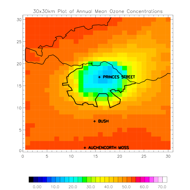
Figure 6: 30 x 30 km annual mean simulated ozone concentration for Edinburgh.

The output for the annual average ozone concentration at Bush and Auchencorth are in excellent agreement with the annual average observed ozone concentration for the two sites in 1995-97 - see Table 6. It should be remembered, however, that Auchencorth values were used to determine the upwind boundary conditions.

SITE	MODELLED	OBSERVED
Princes Street	16$\mu$g m-3	31$\mu$g m-3
Bush	54$\mu$g m-3	53$\mu$g m-3
Auchencorth Moss	55$\mu$g m-3	54$\mu$g m-3

Table 6: Annual average ozone concentrations at the three monitoring sites - both modelled and observed results

However, at Princes Street the agreement is not nearly so good with the modelled value only about half the observed average; but the model value is the average concentration over the whole 1x1km grid-square that the monitoring station is in. In reality the concentration varies greatly across the grid square and the observations may be taken at a site where the concentration is not representative of the whole area. This is in contrast to the Auchencorth site, where the uniformity of the landscape and the lack of local sources makes it representative of a large area. It might though be expected that the observations, particularly at Princes Street, would be smaller than the modelled results as they are taken within a few metres of the road itself. The position of the monitoring site though is slightly unusual in that it is positioned within a garden that is at a lower level than the road. The model treats the entire domain as it it were flat and is unable to recreate the effects of such topographic detail. However, with the height of the monitoring inlet being 4m above the surrounding ground, it is almost on the same level as the adjacent road and thus should still be sampling air that is depleted in ozone. It appears that the model is under-estimating ozone concentrations within urban areas.

The spatial extent of ozone depletion greater than 5$\mu$g m^-3 from the background (Auchencorth) value of 55$\mu$g m^-3 is fairly limited on an annual-average basis. The 50$\mu$g m^-3 isopleth extends only a few kilometres outside the city boundary - reaching a maximum distance of approximately 10km downwind of the dominant wind direction (see Tables 1 and 2), to the north-east. Areas with concentrations less than 45$\mu$g m^-3 (a 20$\%$ depletion) are mainly confined within the city boundary and, due to the prevailing wind from the southwest, out over the Firth of Forth to the north-east. Only an area of approximately 8x8km, just offset from the city centre is depleted by more than 50%.

6 Modelling Vertical and Temporal Variations in Edinburgh’s Ozone Concentrations

6.1 Vertical Section of Ozone Concentrations Through Edinburgh

Figure 7 is the 30x30km plot of ozone concentrations for midday in December.

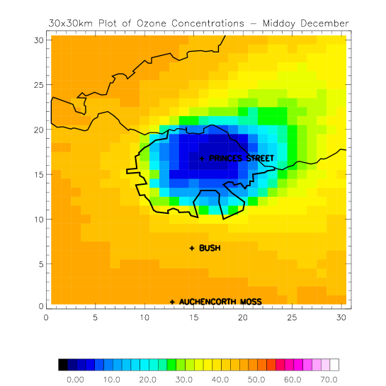
Figure 7: 30 x 30 km simulated ozone concentration for Edinburgh - December, 1200h.

The city centre ozone concentration is less than 5$\mu$g m^-3 with the Bush and Auchencorth concentrations being 46 and 48$\mu$g m^-3 respectively. Depletion greater than 20$\%$ ($\it{ie.}$ less than 35$\mu$g m^-3) is again mainly confined to the city and areas to the north and east, out over the Firth of Forth.

Figure 8 is a north-south vertical section (0-150m) through the 1200hrs December ozone concentration field - passing through Princes Street. Above 100m there is little detail of the city below that can be seen at all (except for some jagged peaks that are artefacts of the plotting program used). It can be seen that the section is skewed with lower concentration spread out towards the north - this can also be seen in the two-dimensional plot (Figure 7). Concentrations of less than 25$\mu$g m^-3, $\it{ie.}$ 50% depletion, are restricted to below 20m. At nighttime, this would be even lower - just a few metres above the ground.

6.2 Diurnal Variation of Ozone Concentrations

Diurnal plots of ozone concentrations at Princes Street and Bush for December have been made by calculating the hourly ozone concentrations for 24 hours. These are plotted in Figure 9 and are compared with observational data obtained from the two monitoring stations (hourly averages) from 3 years (1995-97). Any day with missing data for any of the species were ignored; however overall data capture was greater than $90\%$.

As can be seen from the diurnal variation plot, the values at Bush generated by the model are closer to the observed average values (as expected due to the definition of the upwind perimeter concentrations) than those at Princes Street but the pattern of the diurnal variation produced by the model at Princes Street more closely resembles the observations, despite a systematic under-estimation of 10-20$\mu$g m^-3.

At Princes Street, the only feature of the modelled variation that doesn’t correspond well with the observed values is in the middle of the day when there is a peak in the concentration from the minima during the dawn and dusk rush hours. This is due to the increased mixing in the day in the model from the increased insolation. The reason that the modelled values are on average 10$\mu$g m^-3 less than those observed may be due to one or more of several reasons:

• The emission used in the model may not be appropriate for the locality.

• Vertical mixing may be underestimated. No account is taken of the heat island effect.

• It is likely that the complex mixing processes taking place within the street canyons are not adequately represented.

• Mixing depends on stability, which is determined only by external conditions (cloud cover and wind speed) at the time. There is no ”memory” of preceeding conditions.

The observed values at Bush are lower than those produced by the model and show that this site is also influenced by the Edinburgh rush hour. There are two roads within 500m of the site that carry substantial traffic into and out of the city in the morning and evening and the corresponding dips in the ozone concentration at 0900 and 1700hours can be attributed to this. There appears to be a discontinuity in the modelled data in the very middle of the day, where the concentration dips instead of rising to a small peak at midday as happens at Princes Street. This may be due to the ozone deposition velocity during the day over rural areas reaching such a value that depletion of ozone at the surface exceeds the mixing down of ozone rich air from aloft. The small deposition velocity and greater mechanical turbulence over the city ensure that this does not occur at the Prices Street site.

7 Conclusions

The Lagrangian column model has been used in this study to produce a series of one- and two-dimensional maps of surface ozone concentrations under a variety of meteorological conditions.

One-dimensional straight-line trajectories under average summertime boundary-layer conditions show a depletion of surface ozone over an urban area of $40\%$ in daytime with a downwind recovery to approximately $80\%$ of upwind rural values at 20km and $100\%$ depletion with an eventual recovery to $50\%$ downwind at night. Similar trajectories run in winter, with lower insolation levels and greater mean wind-speeds show $90\%$ of the surface ozone is depleted in both daytime and nighttime conditions. At nighttime, the downwind recovery to $60\%$ of the upwind concentration is faster than the daytime recovery.

Vertical profiles upwind, within and downwind of the city show how the concentration gradient in the lowest 150m increases as the column passes over the city and then decreases again downwind as the loss of ozone is evenly spread through the layers. The upwind and downwind profiles have very similar shapes - at midday in June the difference between the two profiles is approximately 12$\mu$g m^-3 throughout the profile. A vertical section through the simulated city for December shows that $50\%$ depletion is restricted to the lowest 20m of the vertical column and that at 100m altitude, the effects of the city on ozone concentrations are barely discernible.

Two-dimensional maps of annual mean surface ozone concentrations show that the depletion of ozone by a city is restricted to very close to the urban area. A depletion of $20\%$ of the background ozone in a simulated Edinburgh only extends beyond the city boundaries downwind of the prevailing wind direction while $50\%$ depletion is completely confined within the city boundaries.

At this stage we can revisit the omission of ozone generation from the model formulation. Typical gradients of ozone concentration around the city boundary are 20-30$\mu$g m^-3 per 5km (see Fig. 6). Observations of ozone generation rates are typically at least an order of magnitude less than this (e.g. (?)), so that patterns of concentration would not be significantly affected by its inclusion.

The diurnal cycle of ozone concentrations at urban and rural sites has been compared with monitoring site data. The model recreates the shape of the diurnal cycle well - but consistently underestimates the city-centre surface concentrations. This could be due to underestimating atmospheric turbulence, overestimating emissions or the fact that the single point of the monitoring station does not accurately represent the full 1x1km grid-square. The model also overestimates the concentrations at the rural site, which is more dependent on the emissions from local roads than used in the model.

8 Acknowledgements

The authors acknowledge Dr Rod Singles and Dr Helen ApSimon et al. for the use of the TERN model and their expert advice. Ms Mhairi Coyle, Dr Chris Flechard (C.E.H., Edinburgh), Dr Justin Goodwin (NETCen) and Edinburgh City Council Roads Department are thanked for supplying data. J. Nicholson was in receipt of a Natural Environment Research Council studentship.