Complex Scaling of the Faddeev Equations

Abstract

In this work we compare two different approaches to calculation of the three-body resonances on the basis of Faddeev differential equations. The first one is the complex scaling approach. The second method is based on an immediate calculation of resonances as zeros of the three-body scattering matrix continued to the physical sheet.

, ,

1 Introduction

The complex scaling method [1, 2] invented in early 70-s remains one of the most effective approaches to calculation of resonances in few-body systems. This method is applicable to an $N$-body problem in the case where inter-particle interaction potentials are analytic functions of coordinates. The complex scaling gives a possibility to rotate the continuous spectrum of an $N$-body Hamiltonian in such a way that certain sectors of unphysical sheets neighboring the physical one turn into a part of the physical sheet for the resulting non-selfadjoint operator. Resonances appear to be complex eigenvalues of this operator [1, 2] while the binding energies stay fixed during the scaling transformations. Therefore, when searching for the resonances within the complex scaling approach one may apply the methods which are usually employed to locate the binding energies. Some reviews of the literature on the complex scaling and its many applications can be found, in particular, in [4, 5, 6]. Here we only mention that there is a rigorous mathematical proof [3] that for a rather wide class of interaction potentials the resonances given by the complex scaling method coincide with the “true scattering resonances”, i. e. the poles of the analytically continued scattering matrix in the unphysical sheets.

Along with the complex scaling, various different methods are also used for calculations of the resonances. Among the methods developed to calculate directly the scattering-matrix resonances we, first, mention the approach based on the momentum space Faddeev integral equations [7, 8] (see, e. g., Ref. [9] and references cited therein). In this approach one numerically solves the equations continued into an unphysical sheet and, thus, the three-body resonances arise as the poles of the continued T-matrix. Another approach to calculation of the scattering-matrix resonances is based on the explicit representations [10, 11] for the analytically continued T- and S-matrices in terms of the physical sheet. From these representations one infers that the three-body resonances can be found as zeros of certain truncations of the scattering matrix only taken in the physical sheet. Such an approach can be employed even in the coordinate space [11, 12].

To the best of our knowledge there are no published works applying the complex scaling to the Faddeev equations. Therefore, we consider the present investigation as a first attempt undertaken in this direction. However, the purpose of our work is rather two-fold. On the one hand, we make the complex scaling of the Faddeev differential equations. On the other hand we compare the complex scaling method with the scattering-matrix approach suggested in [11, 12]. We do this making use of both the approaches to examine resonances in a model system of three bosons having the nucleon masses and in the three-nucleon ($nnp$) system itself.

2 Formalism

First, we recall that, after the scaling transformation, the three-body Schrödinger operator reads as follows [1, 2, 3]

$$H(\vartheta)=-{\rm e}^{-2\vartheta}\Delta_{X}+\sum_{\alpha=1}^{3}V_{\alpha}({\rm e}^{\vartheta}x_{\alpha})$$ (1)

where $\vartheta={\rm i}\theta$ is the scaling parameter with $\theta\in{\mathbb{R}}$. By $\Delta_{X}$ we understand the six–dimensional Laplacian in $X\equiv({\bf x}_{\alpha},{\bf y}_{\alpha})$ where ${\bf x}_{\alpha},{\bf y}_{\alpha}$ are the standard Jacobi variables, $\alpha=1,2,3$. Notation $V_{\alpha}$ is used for the two-body potentials which are assumed to depend on $x_{\alpha}=|{\bf x}_{\alpha}|$ but not on $\widehat{{\bf x}}_{\alpha}={\bf x}_{\alpha}/x_{\alpha}$.

The corresponding scaled Faddeev equations which we solve read

$${[-{\rm e}^{-2\vartheta}\Delta_{X}+v_{\alpha}({\rm e}^{\vartheta}x_{\alpha})-z]\Phi^{(\alpha)}(z;X)+V_{\alpha}({\rm e}^{\vartheta}x_{\alpha})\sum_{\beta\neq\alpha}\Phi^{(\beta)}(z;X)=f_{\alpha}(X),}$$

$$\qquad\qquad\qquad{\alpha=1,2,3.}$$ (2)

Here $f=(f_{1},f_{2},f_{3})$ is an arbitrary three-component vector with components $f_{\alpha}$ belonging to the three-body Hilbert space $L_{2}({\mathbb{R}}^{6})$.

The partial-wave version of the equations (2) for a system of three identical bosons at the zero total angular momentum $L=0$ reads

$${{\rm e}^{-2{\rm i}\theta}}H_{0}^{(l)}\Phi_{l}(z;x,y)-z\,\Phi_{l}(z;x,y)+V({{\rm e}^{{\rm i}\theta}}x)\Psi_{l}(z;x,y)={{f^{(l)}(x,y)}}$$ (3)

where $x>0$, $y>0$ and $H_{0}^{(l)}$ denotes the partial-wave kinetic energy operator,

$$H_{0}^{(l)}=-\displaystyle\frac{\partial^{2}}{\partial x^{2}}-\displaystyle\frac{\partial^{2}}{\partial y^{2}}+l(l+1)\left(\displaystyle\frac{1}{x^{2}}+\displaystyle\frac{1}{y^{2}}\right)\,,\qquad l=0,2,4,\ldots,$$

while $\Psi_{l}$ stands for the partial-wave component of the total wave function,

$$\Psi_{l}(z;x,y)=\Phi_{l}(z;x,y)+\sum_{l^{\prime}}\int_{-1}^{+1}d\eta\,h_{ll^{\prime}}(x,y,\eta)\,\Phi_{l^{\prime}}(z;x^{\prime},y^{\prime})\,.$$ (4)

Here, $x^{\prime}=\sqrt{\frac{1}{4}\,x^{2}+\frac{3}{4}\,y^{2}-\frac{\sqrt{3}}{2}\,xy\eta}$ and $y^{\prime}=\sqrt{\frac{3}{4}\,x^{2}+\frac{1}{4}\,y^{2}+\frac{\sqrt{3}}{2}\,xy\eta}$. Explicit expression for the geometric function $h_{ll^{\prime}}(x,y,\eta)$ can be found, e. g., in [8].

The partial-wave equations (3) are supplied with the boundary conditions

$$\left.\Phi_{l}(z;x,y)\right|_{x=0}=0\quad\mbox{and}\quad\left.\Phi_{l}(z;x,y)\right|_{y=0}=0.$$ (5)

For compactly supported inhomogeneous terms $f^{(l)}(x,y)$ the partial-wave Faddeev component $\Phi_{l}(z;x,y)$ also satisfies the asymptotic condition

$$\begin{array}[]{lll}\Phi_{l}(z;x,y)&=&\delta_{l0}\psi_{d}({{\rm e}^{{\rm i}\theta}}x)\exp({\rm i}\sqrt{z-\epsilon_{d}}\,\,{{\rm e}^{{\rm i}\theta}y})\left[{\rm a}_{0}(z)+o\left(y^{-1/2}\right)\right]\\ &+&\displaystyle\frac{\exp({\rm i}\sqrt{z}\,\,{{\rm e}^{{\rm i}\theta}}\rho)}{\sqrt{\rho}}\left[A_{l}(z;y/x)+o\left(\rho^{-1/2}\right)\right],\end{array}$$ (6)

For simplicity it is assumed in this formula that the two-boson subsystem has only one bound state with the energy $\epsilon_{d}$, and $\psi_{d}(x)$ represents its wave function. The values of ${\rm a}_{0}$ and $A_{l}(y/x)$ are the main asymptotical coefficients effectively describing the contributions to $\Phi_{l}$ from the elastic $(2+1\to 2+1)$ and breakup $(2+1\to 1+1+1)$ channels, respectively. Hereafter, by $\sqrt{\zeta}$, $\zeta\in\mathbb{C}$, we understand the main (arithmetic) branch of the function $\zeta^{1/2}$.

In the scaling method a resonance is looked for as the energy $z$ which produces a pole to the quadratic form

$${Q(\theta,z)=\left<\left[H_{F}(\theta)-z\right]^{-1}f,f\right>}\,$$

where $H_{F}(\theta)$ is the non-selfadjoint operator resulting from the complex-scaling transformation of the Faddeev operator. The latter operator is just the operator constituted by the l. h. s. parts of Eqs. (2). The resonance energies should not, of course, depend on the scaling parameter $\theta$ and on the choice of the terms $f^{(l)}(x,y)$.

In the scattering-matrix approach we solve the same partial-wave Faddeev equations (3) with the same boundary conditions (5) and (6) but for $\theta=0$ and

$$f^{(l)}(x,y)=-V(x)\int_{-1}^{+1}d\eta\,h_{l0}(x,y,\eta)\,\psi_{d}(x^{\prime})\sin(\sqrt{z-\epsilon_{d}}\,y^{\prime}).$$

The resonances are looked for as zeroes of the truncated scattering-matrix (see [12] for details) ${\rm s}_{0}(z)=1+2{\rm i}{\rm a}_{0}(z)$, where the $(1+1\to 1+1)$ elastic scattering amplitude ${\rm a}_{0}(z)$ for complex energies $z$ in the physical sheet is extracted from the asymptotics (6).

For numerical solution of the boundary-value problem (3 – 6) we employ its finite-difference approximation in the hyperradius-hyperangle coordinates. A detail description of the finite-difference algorithm used can be found in Ref. [13].

3 Results

In the table we present our results obtained for a complex-scaling resonance in the model three-body system which consists of identical bosons having the nucleon mass. To describe interaction between them we employ a Gauss-type potential of Ref. [12]

$$V(x)=V_{0}\exp[-\mu_{0}x^{2}]+V_{b}\exp[-\mu_{b}(x-x_{b})^{2}]$$

with $V_{0}=-55$ MeV, $\mu_{0}=0.2$ fm^-2, $x_{b}=5$ fm, $\mu_{b}=0.01$ fm^-2 and $V_{b}=1.5$. The figures in the table correspond to the roots of the inverse function $[Q(\theta,z)]^{-1}$ for $L=0$ and $l=0$ only taken into account. In the present calculation we have taken up to 400 knots in both hyperradius and hyperangle variables while for the cut-off hyperradius we take 40 fm. One observes from the table that the position of the resonance depends very weakly on the scaling parameter $\theta$ which confirms a good numerical quality of our results. We compare the resonance values of the table to the resonance value $z_{\rm res}=-5.952-0.403\,{\rm i}$ MeV obtained for the same three-boson system with exactly the same potentials but in the completely different scattering-matrix approach of Ref. [12]. We see that, indeed, both the complex scaling and the scattering matrix approaches give the same result.

$\theta$	$z_{\rm res}$ (MeV)	$\theta$	$z_{\rm res}$ (MeV)
0.25	$-5.9525-0.4034\,{\rm i}$	0.50	$-5.9526-0.4032\,{\rm i}$
0.30	$-5.9526-0.4033\,{\rm i}$	0.60	$-5.9526-0.4033\,{\rm i}$
0.40	$-5.9526-0.4032\,{\rm i}$	0.70	$-5.9526-0.4034\,{\rm i}$

We also watched the trajectory of the above resonance when the barrier amplitude $V_{b}$ varied (see. Fig. 1). While the complex scaling method was applicable it gave practically the same positions for the resonance. For the barrier amplitudes $V_{b}$ smaller than 1.0 only the scattering-matrix approach allows to locate the resonance (which finally, for $V_{b}<0.85$, turns into a virtual level).

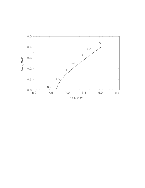
Figure 1: Trajectory of the resonance $z_{\rm res}$ in the model system of three bosons with the nucleon masses. Values of the barrier $V_{b}$ in MeV are given near the points marked on the curve.

As to the $nnp$ system in the $S$ – state where we employed the MT I–III [14] potential model, both the methods applied give no resonances on the two-body unphysical sheet (see [12]). Moreover, we have found no resonances in the part of the three-body sheet accessible via the complex scaling method. Thus, at least in the framework of the MT I–III model we can not confirm the experimental result of Ref. [16] in which the point $-1.5\pm 0.3-{\rm i}(0.3\pm 0.15)$ MeV was interpreted as a resonance corresponding to an exited state of the triton ³H.

The triton virtual state can be only calculated within the scattering-matrix method but not in the scaling approach. Our present improved scattering-matrix result for the triton virtual state is $-2.690$ MeV (i. e. the virtual level lies 0.47 MeV below the two-body threshold). This result has been obtained with the MT I-III potential on a grid having 1000 knots in both hyperradial and hyperradial variables and with the value of cut-off hyperradius equal to 120 fm. Notice that some values for the virtual-state energy obtained by different authors can be found in [9] and all of these values are about 0.5 MeV below the two-body threshold.

References

- [1] E. Balslev, J. M. Combes, Commun. Math. Phys., 22 (1971), 280.
- [2] M. Reed, B. Simon, Methods of modern mathematical physics. IV: Analysis of operators, Academic Press, N. Y., 1978.
- [3] G. A. Hagedorn, Comm. Math. Phys. 65 (1979), 81.
- [4] Y. K. Ho, Phys. Rep. 99 (1983), 3; Chin. J. Phys. 35 (1997), 97.
- [5] B. R. Junker, Adv. Atom. Mol. Phys. 18 (1982), 208.
- [6] W. P. Reinhard, Ann. Rev. Phys. Chem. 33 (1982), 223.
- [7] L. D. Faddeev, Mathematical aspects of the three–body problem in quantum mechanics, Israel Program for Scientific Translations, Jerusalem, 1965.
- [8] L. D. Faddeev, S. P. Merkuriev, Quantum scattering theory for several particle systems, Kluwer Academic Publishers, Dorderecht, 1993.
- [9] K. Möller, Yu. V. Orlov, Fiz. Elem. Chast. At. Yadra. 20 (1989), 1341 (Russian).
- [10] A. K. Motovilov, Theor. Math. Phys. 95 (1993), 692.
- [11] A. K. Motovilov, Math. Nachr. 187 (1997), 147.
- [12] E. A. Kolganova, A. K. Motovilov, Phys. Atom. Nucl. 60 (1997), 235.
- [13] E. A. Kolganova, A. K. Motovilov, S. A. Sofianos, J. Phys. B. 31 (1998), 1279.
- [14] R.A.Malfliet, J.A.Tjon, Nucl. Phys. A 127 (1969), 161.
- [15] Yu. V. Orlov, V. V. Turovtsev, JETP 86 (1984), 1600 (Russian).
- [16] D. V. Alexandrov et. al., JETP Lett. 59 (1994), 320 (Russian).