[

On a correspondence between classical and quantum particle systems

Abstract

An exact correspondence is established between a $N$-body classical interacting system and a $N-1$-body quantum system with respect to the partition function. The resulting quantum-potential is a $N-1$-body one. Inversely the Kelbg potential is reproduced which describes quantum systems at a quasi-classical level. The found correspondence between classical and quantum systems allows also to approximate dense classical many body systems by lower order quantum perturbation theory replacing Planck’s constant properly by temperature and density dependent expressions. As an example the dynamical behaviour of an one - component plasma is well reproduced concerning the formation of correlation energy after a disturbance utilising solely the analytical quantum - Born result for dense degenerated Fermi systems. As a practical guide the quantum - Bruckner parameter $r_{s}$ has been replaced by the classical plasma parameter $\Gamma$ as $r_{s}\approx 0.3\Gamma^{3/2}$.

]

Several hints in recent literature conjecture that there seem to exist a correspondence between quantum systems and higher dimensional classical systems. The authors of [1] argue that a higher dimensional classical non-Abelian gauge theory leads to a lower dimensional quantum field theory in the sense of chaotic quantisation. The correspondence has been achieved by equating the temperature characterising chaotization of the higher dimensional system with $\hbar$ of the lower dimensional system by

$$\hbar=aT.$$ (1)

Recalling imaginary time evolution as a method to calculate correlated systems in equilibrium such correspondence seems suggestible. We will find a similar relation as a best fit of quantum - Born calculations to dense interacting classical systems.

In condensed matter physics it is a commonly used trick to map a two - dimensional classical spin system onto a one - dimensional quantum system [2]. This suggests that there might exist a general relation between classical and higher dimensional quantum systems. We will show that a classical many body system can be equally described by a quantum system with one particle less in the system but with the price of complicated nonlocal potential. This can be considered analogously to the Bohm interpretation of quantum mechanics [3] where the Schroedinger equation is rewritten in a Hamilton-Jacobi equation but with a nonlocal quantum potential.

Another hint towards a correspondence between classical and quantum systems was found recently in [4] where it was achieved to define a Lyapunov exponent in quantum mechanics by employing the marginal distribution which is a representation of Wigner function in a higher dimensional space. Since the Lyapunov exponent is essentially a concept borrowed from classical physics this finding points also in the direction that there exists a correspondence between quantum systems and higher dimensional classical systems.

On the opposite side there are systematic derivations of constructing effective classical potentials such that the many body quantum system is described by the classical system. An example is the Kelbg potential for Coulomb systems [5, 6, 7, 8]

$$V^{\rm Kelbg}_{12}(r)={e_{1}e_{2}\over r}\left(1-{\rm e}^{-r^{2}/l^{2}}+\sqrt{\pi}{r\over l}{\rm erfc}\left({r\over l}\right)\right)$$ (2)

with $l^{2}=\hbar^{2}/2\mu T$ and $1/\mu=1/m_{1}+1/m_{2}$ describing the two-particle quantum Slater sum correctly by a classical system. Improvements and systematic applications can be found in [9, 10, 11].

Here in this paper it should be shown that a classical $N$-particle system can be mapped exactly on a quantum $N-1$-particle system with respect to the partition function. Though the resulting effective $N-1$ body quantum potential is highly complex it can lead to practical applications for approximating strongly correlated classical systems. In the thermodynamical limit it means that the dense classical system can be described alternatively by a quantum system with properly chosen potential.

This finding suggests that the quantum calculation in lowest order perturbation might be suitable to derive good approximations for the dense classical system. This is also motivated by an intuitive picture. Assume we have a dense interacting classical plasma system. Then the correlations will restrict the possible phase space for travelling of one particle considerably like in dense Fermi systems at low temperatures where the Pauli exclusion principle restrict the phase space for scattering. Therefore we might be able to describe a dense interacting classical system by a perturbative quantum calculation when properly replacing $\hbar$ by density and temperature expressions. Indeed we will demonstrate in a one - component plasma system that even the time evolution and dynamics of a very strongly correlated classical system can be properly approximated by quantum - Born calculations replacing the quantum parameters by proper classical ones.

Let us now start to derive the equivalence between classical and quantum systems by rewriting the classical N-particle partition function. The configuration integral reads

$$Q_{N}(\beta)=\int dx_{1}...dx_{N}\prod\limits_{i<j}^{N}(1+f_{ij})$$ (3)

where we used Meyer’s graphs $f_{ij}=\exp{(-\beta u_{ij}(x_{i}-x_{j}))}-1$ with the interaction potential $u_{ij}(x_{i}-x_{j})$ of the classical particles and the inverse temperature $\beta$. It is now of advantage to consider the modified configuration integral

$$\tilde{Q}_{N}(\beta)=Q_{N}(2\beta)$$ (4)

$$=\int dx_{1}...dx_{N}dx_{1}^{\prime}...dx_{N}^{\prime}\delta(x_{1}-x_{1}^{\prime})...\delta(x_{N-1}-x_{N-1}^{\prime})$$ (5)

$$\matrix{\times&(1+f_{12})(1+f_{13})(1+f_{14})...(1+f_{1N})\cr\times&(1+f_{21^{\prime}})(1+f_{23})(1+f_{24})...(1+f_{2N})\cr\times&......\cr\times&(1+f_{N1^{\prime}})(1+f_{N2^{\prime}})(1+f_{N3^{\prime}})...(1+f_{NN-1^{\prime}})}$$ (6)

such that a quadratic schema in $f_{ij^{\prime}}$ appears. Now we assume a complete set of $N-1$ particle wave functions $\Psi_{n_{N-1}}$ such that

$$\delta(x_{1}-x_{1}^{\prime})...\delta(x_{N-1}-x_{N-1}^{\prime})$$ (7)

$$=\sum\limits_{i_{1}..i_{N-1}}\Psi^{*}_{i_{1}..i_{N-1}}(x_{1}^{\prime}...x_{N-1}^{\prime})\Psi_{i_{1}..i_{N-1}}(x_{1}...x_{N-1})$$ (8)

with some ”quantum numbers” $\{i\}$ characterising the state. Further we propose the following eigenvalue problem defining the wave function

$$\int dx_{1}\prod\limits_{j=2}^{N}(1+f_{1j})\Psi_{i_{1}..i_{N-1}}(x_{1}...x_{N-1})$$ (9)

$$\qquad\qquad=V{\rm e}^{-\varepsilon_{\{i\}}}\Psi_{i_{2}..i_{N-1}i_{1}}(x_{2}...x_{N})$$ (10)

with the system volume $V$. This allows to calculate the configurational integral (6) exactly by successively integrating $x_{1}...x_{N}$

$$\tilde{Q}_{N} (\beta)$$ (11)

$$= \sum\limits_{i_{1}..i_{N-1}}\int dx_{1}...dx_{N}dx_{1}^{\prime}...dx_{N-1}^{\prime}\Psi^{*}_{i_{1}..i_{N-1}}(x_{1}^{\prime}...x_{N-1}^{\prime})$$ (14)

$$\times\Psi_{i_{1}..i_{N-1}}(x_{1}...x_{N-1})$$

$$\matrix{\times&(1+f_{12})(1+f_{13})(1+f_{14})...(1+f_{1N})\cr\times&(1+f_{21^{\prime}})(1+f_{23})(1+f_{24})...(1+f_{2N})\cr\times&......\cr\times&(1+f_{N1^{\prime}})(1+f_{N2^{\prime}})(1+f_{N3^{\prime}})...(1+f_{NN-1^{\prime}})}$$

$$= \sum\limits_{i_{1}..i_{N-1}}\int dx_{1}^{\prime}...dx_{N-1}^{\prime}\Psi^{*}_{i_{1}..i_{N-1}}(x_{1}^{\prime}...x_{N-1}^{\prime})$$ (16)

$$\times V^{N}{\rm e}^{-N\varepsilon_{\{i\}}}\Psi_{i_{1}..i_{N-1}}(x_{1}^{\prime}...x_{N-1}^{\prime})$$

$$= V^{N}\sum\limits_{i_{1}..i_{N-1}}{\rm e}^{-N\varepsilon_{\{i\}}}.$$ (17)

This establishes already the complete proof that we can map a classical $N$-body system on a $N-1$-body quantum system since (10) is the eigenvalue problem of a $N-1$-body Schroedinger equation. To see this we can consider a wavefunction $\xi$ built from the Fouriertransform of $\tilde{\Psi}$

$$\xi(p_{1}...p_{N-1},t)={\rm e}^{-{i\over\hbar}\sum\limits_{i=1}^{N-1}{p_{i}^{2}\over 2m_{i}}t}\tilde{\Psi}_{i_{1}...i_{N-1}}(p_{1}...p_{N-1})$$ (18)

which obeys the $N-1$-particle Schroedinger equation

$$\left(i\hbar{\partial\over\partial t}-\sum\limits_{i}^{N-1}{p_{i}^{2}\over 2m_{i}}-\tilde{U}\right)\xi=E_{N-1}\xi$$ (19)

with $E_{N-1}\propto V{\rm e}^{-\varepsilon_{\{i\}}}$ and we rewrote the left hand side of (10) as quantum potential

$$<x_{1}i_{1}...x_{N-1}i_{N-1}|U|x_{1}^{\prime}i_{1}^{\prime}...x_{N-1}^{\prime}i_{N-1}^{\prime}>$$ (20)

$$= {\rm e}^{{\beta}[u_{12}(x_{1}^{\prime}-x_{1})+...+u_{1N}(x_{1}^{\prime}-x_{N-1})]}$$ (22)

$$\times\Omega\delta(x_{1}-x_{2}^{\prime})...\delta(x_{N-2}-x_{N-1}^{\prime})\delta_{i_{1}^{\prime},i_{1}}...\delta_{i_{N-1}^{\prime},i_{N-1}}.$$

The resulting equivalent quantum potential (22) is a $N-1$-body nonlocal potential with respect to the coordinates but depends on $N$ strength function parameter (e.g. charges). Therefore we have casted a classical $N$-body problem into a nonlocal quantum $N-1$ body problem. One could easily give also a symmetrised or anti-symmetrised form of the potential using symmetries of the wave function and permuting coordinates of (22) respectively. We do not need it here since we will restrict to applications neglecting exchange correlations further on.

While the above correspondence holds for any particle number and might be useful to find solvable models for classical three - body problems, we will consider in the following many - body systems. First let us invert the problem and search for an effective classical potential approximating quantum systems. This should us lead to the known Kelbg-potential (2). For this purpose we assume a quantum system described in lowest approximation by a Slater determinant or a complete factorisation of the many - body wave function into single wave function $\Psi_{i_{1}...i_{N}}(x_{1}...x_{N})=\phi_{i_{1}}...\phi_{i_{N}}$. We neglect for simplicity exchange correlations in the following. The corresponding eigenvalue equation for $\phi$ itself one can obtain from (10) or (19) by multiplying with $\Psi_{i_{2}..i_{N-1}}^{*}(x_{2}...x_{N-1})$ and integrate over $x_{2}...x_{N-1}$. To see the generic structure more clearly we better calculate the correlation energy by multiplying (10) or (19) by $\Psi_{i_{2}..i_{N-1}i_{1}}^{*}(x_{2}...x_{N})$ and integrating over $x_{2}...x_{N}$. This provides also the eigenvalue $\epsilon_{\{i\}}$ and leads easily to approximations for the partition function (3). To demonstrate this we choose the lowest order approximation taking identical plane waves for $\phi$. Than the pressure can be obtained from the partition function $Q_{N}$ via (17)

$$P\!=\!T{\partial\over\partial V}\ln Q_{N}\!=\!T\left({N\over V}\!-\!{N(N\!-\!2)\over V^{2}}\int\!dr\!\left(\!{\rm e}^{\!-\!\beta u(r)/2}\!-\!1\!\right)\right)$$ (23)

where $V$ is the volume of the system. We recognise the standard second virial coefficient for small potentials while for higher order potential the factor $1/2$ appears in the exponent instead as a pre-factor indicating a different partial summation of diagrams due to the schema behind (17) and (19).

To go beyond the plane wave approximation we multiply (10) by $\Psi_{i_{2}..i_{N-1}i_{1}}^{*}(x_{2}...x_{N})$ and the kinetic part of the statistical operator before integrating over $x_{2}...x_{N}$. This means we create an integral over the $N-1$ particle density operator and the potential (22) which together represents the correlation energy. This expression is a successive convolution between the cluster graphs $f_{ij}$ and the relative two - particle correlation function $\rho_{i_{1}i_{2}}(x_{1}-x_{2})$. The resulting mean correlation energy density reads

$${U\over V}\!=\!\sum\limits_{\{i\}}\int{dy_{1}\!...\!dy_{N-1}\over V^{N-1}}\rho_{i_{1}i_{2}}(y_{1})\rho_{i_{2}i_{3}}(y_{2})...\rho_{i_{N-1}i_{1}}(y_{N-1})$$ (25)

$$\times(1\!-\!f_{12}(y_{1}))(1\!-\!f_{13}(y_{1}\!+\!y_{2}))...(1\!-\!f_{1N}(y_{1}\!+\!...\!+\!y_{N-1}))$$ (26)

$$\approx\sum\limits_{\{i\}}\int{dy_{1}\!...\!dy_{N-1}\over V^{N-1}}\rho_{i_{1}i_{2}}(y_{1})\!...\!\rho_{i_{N-1}i_{1}}(y_{N-1})$$ (27)

$$\times u_{12}(y_{1})u_{13}(y_{1}\!+\!y_{2})\!...\!u_{1N}(y_{1}\!+\!...\!+\!y_{N-1})+...$$ (28)

in dimensionless units where all other cluster expansion terms lead either to lower mean field or disconnected terms. While these terms can be calculated as well we restrict to the highest order convolutions in the correlation energy (28) which have now the structure of mean correlation energy $U/V=\sum\limits_{i_{1}i_{2}}\int{dx\over V}\rho_{i_{1}i_{2}}(x)V^{\rm eff}_{12}$ with a classical effective potential $V^{\rm eff}_{12}$

$$V^{\rm eff}_{2}(r) \propto \sum\limits_{3}\int{dx_{1}\over V}\rho_{12}(x_{1})u_{12}(x_{1})u_{23}(x_{1}+r)$$ (29)

$$V^{\rm eff}_{3}(r) \propto \sum\limits_{34}\int{dx_{1}dx_{2}\over V^{2}}\rho_{12}(x_{1})u_{12}(x_{1})u_{13}(x_{1}+x_{2})$$ (32)

$$\qquad\qquad\times\rho_{23}(x_{2})u_{34}(x_{1}+x_{2}+r)$$

$$...$$

where the two-particle, three-particle etc. approximation can be given. In equilibrium the nondegenerate correlation function reads $[l^{2}=\hbar^{2}/\mu T=\lambda^{2}/2\pi]$

$$\rho_{i_{1}i_{2}}(x_{1}\!-\!x_{2})\! = \!\!\int\!{dp\over(2\pi\hbar)^{3}}{\rm e}^{ipr/\hbar}\lambda^{3}{\rm e}^{-\beta{p^{2}\over 2\mu}}={\rm e}^{-r^{2}/l^{2}}.$$ (33)

Using the Coulomb potential $u\propto 1/r$ we obtain from the two-particle approximation (29) just the Kelbg potential (2). The three - particle approximation (32) can be calculated as well and reads $[x=r/l]$

$$V^{\rm eff}_{3}\sim{1\over x}\left({\rm erf}^{2}\left({x\over\sqrt{2}}\right)\!+\!{2^{3/2}x\over\sqrt{\pi}}\int\limits_{x}^{\infty}{dz\over z}{\rm e}^{-z^{2}/2}{\rm erf}\left({z\over\sqrt{2}}\right)\right).$$ (34)

(35)

The comparison of the third order potential with the Kelbg potential can be seen in figure 1. The third order potential is somewhat less bound than the Kelbg potential.

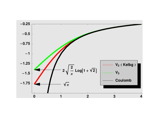
FIG. 1.: The comparison of the Kelbg potential (2) and the third order potential (35) versus $r/l$.

With the schema (32) one can easily integrate higher order approximations as successive convolutions, but with respect to the small differences between (2) and (35) in figure 1 one does not expect much change. Also in principle the degenerate case could be calculated using Fermi-Dirac distributions in (33). But one should then consider also the neglected exchange correlations during factorisation of $\Psi$ as well. Let us summarise that the known effective classical potential describing a quantum system in binary approximation has been recovered by identifying the effective two-particle interaction within the correlation energy.

We want now to proceed to a phenomenological level in that the above correspondence between quantum and classical systems motivates to find good approximations for the dynamics of classical many-body systems by employing quantum-Born approximations. This can be understood by the fact that the Kelbg potential deviates appreciably from the Coulomb one only if the interparticle distance $d$ are smaller than the thermal wave length $\lambda$. In other words for dense classical systems under such conditions we can think of it as a dilute quantum system replacing $\lambda\sim d$. To check this conjecture let us consider an one-component plasma system which is characterised by two values. The classical coupling is described by the plasma parameter $\Gamma={e^{2}\over dT}$ as a ratio of the length where Coulomb energy becomes larger than kinetic energy, ${e^{2}\over T}$, to the interparticle distance or Wigner size radius $d=({3\over 4\pi n})^{1/3}$. Ideal plasmas are found for $\Gamma<<1$ while around $\Gamma=1$ non-ideal effects become important. A second parameter which controls the quantum features is the Bruckner parameter as the ratio of the Wigner size radius to the Bohr radius $a_{B}=\hbar^{2}/me^{2}$. Quantum effects will play a role if $r_{s}\leq 1$. We will consider the situation that the interaction of such system is switched on at initial time. Then the correlations are formed by the system which is seen in an increase of temperature accompanied by the build up of negative correlation energy. This theoretical experiment has been investigated numerically by [12] for classical plasmas with different plasma parameter $\Gamma$.

In [13, 14] we have calculated the formation of such correlations by using quantum kinetic equations in Born approximation. The time dependence of kinetic energy was found at short times to be

$$E_{\rm corr} = -\sum_{ab}\int\frac{dkdpdq}{(2\pi\hbar)^{9}}V^{2}_{\rm D}\frac{1-\cos\left\{{1\over\hbar}t\Delta_{E}\right\}}{\Delta_{E}}$$ (37)

$$\times f^{\prime}_{a}f^{\prime}_{b}(1-f_{a})(1-f_{b})$$

where $f$ are the initial distributions and $\Delta_{E}={k^{2}\over 2m_{a}}+{p^{2}\over 2m_{b}}-{(k-q)^{2}\over 2m_{a}}-{(p+q)^{2}\over 2m_{b}}$. The statical screened Coulomb interaction is $V_{D}(q)=4\pi e^{2}\hbar^{2}/(q^{2}+\hbar^{2}\kappa^{2})$ with the inverse screening length expressed by density $n$ and temperature $T$ as $\kappa^{2}=4\pi e^{2}n/T$ or $\kappa^{2}=6\pi e^{2}n/\epsilon_{f}$ for the high or low temperature limit. For both cases dynamical as well as statical screening it was possible to integrate analytically the time dependent correlation energy (37). This has allowed to describe the time dependence of simulations in the weak coupling limit $\Gamma<1$ appropriately [13]. For stronger coupling $\Gamma\geq 1$ the Born approximation fails since the exact correlation energy of simulation is lower than the first order (Born) result $\kappa e^{2}/2T=\sqrt{3/2}\Gamma^{3/2}$. Moreover there appear typical oscillations as seen in figure 2.

Now we will employ the ideas developed above and will use the quantum Born approximations in the strongly degenerated case to describe the classical strongly correlated system. For strongly degenerated plasmas the time dependence of correlation energy was possible to integrate as well with the result [14] expressed here in terms of plasma parameter $\Gamma$ and quantum Bruckner parameter $r_{s}$ as

$${E_{\rm corr}^{T}(t)-E_{\rm corr}^{0}(t)\over nT} = {1\over(36\pi^{4})^{1/6}}{r_{s}^{3}\over\Gamma}\left({\sin{y\tau}\over y\tau}-1\right)$$ (39)

$$\times\left({1\over b_{l}}{\rm arctan}({1\over b_{l}})+{1\over b_{l}^{2}+b_{l}^{4}}\right)$$

with $b_{l}=\hbar\kappa/2p_{f}=\sqrt{\Gamma}/(48\pi^{2})^{1/6}$, $y\tau=4\epsilon_{f}t/\hbar=(2)^{4/3}\pi^{5/3}3^{5/6}\tau/\sqrt{r_{s}}$ where the time is scaled in plasma periods $\tau=2\pi t/\omega_{p}$. Now we try to fit this quantum result to the simulation using the Bruckner parameter as free parameter. For the available simulations between $1\leq\Gamma\leq 10$ we obtain a best fit

$$r_{s}^{\rm fit}=c\sqrt{3\over 8}\Gamma^{3/2}\qquad c\approx 0.5.$$ (40)

The quality of this fit is illustrated in figure 2 which is throughout the range $1\leq\Gamma\leq 10$. This is quite astonishing since not only the correct classical correlation energy [15] is described but also the correct time dependence i.e. dynamics.

FIG. 2.: The time evolution of a classical one-component plasma after sudden switching of interaction [12] compared to the quantum Born result when the Bruckner parameter is replaced according to (40). The long time equilibrium value is remarkably well reproduced by the quantum - Born result(39).

Let us try to understand what this phenomenological finding means. Using the thermal De Broglie wave length $\lambda^{2}=\hbar^{2}/4mT$ we can rewrite (40) as

$${\lambda^{2}}\approx{d\over\kappa}={d^{2}\over(3\Gamma)^{1/2}}.$$ (41)

In the considered range of $\Gamma=1...10$ we have $(3\Gamma)^{1/4}=1...2$ and the thermal wave length $\lambda$ is found to be nearly equal the interparticle distance $d$ as a best fit of quantum Born calculation to dense classical systems. This is exactly the distance where the Kelbg potential (29) or (2) starts to deviate from the Coulomb potential. In other words we confirm the conjecture that the dense classical system can be described by dilute quantum systems if in the latter systems the thermal wave length is replaced by the interparticle distance. This condition (40) can also be rewritten into the result (1) of literature using the degenerated screening length.

We summarise that in equilibrium we have shown that there exist an exact relation between a $N$-body classical system and a $N-1$-body quantum system. This has allowed to recover the quantum Kelbg potential easily. As practical consequence we suggest to describe the dynamics of dense interacting classical many body systems by the simpler perturbative quantum calculation in degenerate limit replacing properly $\hbar$ by typical classical parameters of the system.

I would like to thank S. G. Chung for numerous discussions and valuable hints.

REFERENCES

- [1] T. S. Biró, S. G. Matinyan, and B. Müller, (2000), hep-th/0010134.
- [2] S. G. Chung, Phys. Rev. B 60, 11761 (1999).
- [3] D. Bohm and B. J. Hiley, Foundations of Physics 14, 255 (1984).
- [4] V. I. Man’ko and R. V. Mendes, Physica D 45, 330 (2000).
- [5] G. Kelbg, Ann. Physik 13, 354 (1964).
- [6] G. Kelbg, Ann. Physik 14, 394 (1964).
- [7] W. Ebeling, H. Hoffmann, and G. Kelbg, Beiträge aus der Plasmaphysik 7, 233 (1967).
- [8] D. Kremp and W. D. Kraeft, Ann. Physik 20, 340 (1968).
- [9] W. D. Kraeft, D. Kremp, W. Ebeling, and G. Röpke, Quantum Statistics of Charged Particle Systems (Akademie Verlag, Berlin, 1986).
- [10] W. D. Kraeft and D. Kremp, Zeit. f. Physik 208, 475 (1968).
- [11] J. Ortner, I. Valuev, and W. Ebeling, Contrib. Plasma Phys. .
- [12] G. Zwicknagel, Contrib. Plasma Phys. 39, 155 (1999).
- [13] K. Morawetz, V. Špička, and P. Lipavský, Phys. Lett. A 246, 311 (1998).
- [14] K. Morawetz and H. Köhler, Eur. Phys. J. A 4, 291 (1999).
- [15] S. Ichimaru, Statistical Plasma Physics (Addison-Wesley Publishing company,, Massachusetts, 1994), p. 57.