Pressure determinations for incompressible fluids and magnetofluids

Abstract

Certain unresolved ambiguities surround pressure determinations for incompressible flows, both Navier-Stokes and magnetohydrodynamic. For uniform-density fluids with standard Newtonian viscous terms, taking the divergence of the equation of motion leaves a Poisson equation for the pressure to be solved. But Poisson equations require boundary conditions. For the case of rectangular periodic boundary conditions, pressures determined in this way are unambiguous. But in the presence of “no-slip” rigid walls, the equation of motion can be used to infer both Dirichlet and Neumann boundary conditions on the pressure $P$, and thus amounts to an over-determination. This has occasionally been recognized as a problem, and numerical treatments of wall-bounded shear flows usually have built in some relatively ad hoc dynamical recipe for dealing with it, often one which appears to “work” satisfactorily. Here we consider a class of solenoidal velocity fields which vanish at no-slip walls, have all spatial derivatives, but are simple enough that explicit analytical solutions for $P$ can be given. Satisfying the two boundary conditions separately gives two pressures, a “Neumann pressure” and a “Dirichlet pressure” which differ non-trivially at the initial instant, even before any dynamics are implemented. We compare the two pressures, and find that in particular, they lead to different volume forces near the walls. This suggests a reconsideration of no-slip boundary conditions, in which the vanishing of the tangential velocity at a no-slip wall is replaced by a local wall-friction term in the equation of motion.

To appear in Journal of Plasma Physics

1 Introduction

It has long been the case that pressure determinations for incompressible flows, both Navier-Stokes and magnetohydrodynamic (MHD), are known to be highly non-local. Taking the divergence of the equation of motion

$$\frac{\partial{\bf v}}{\partial t}+{\bf v}\cdot\nabla{\bf v}=\frac{{\bf j}{\times}{\bf B}}{\rho c}-\nabla P+\nu\nabla^{2}{\bf v},$$ (1)

and using $\nabla\cdot{\bf v}=0$ leaves us with a Poisson equation for the pressure $P$, which is said to function as an equation of state:

$$\nabla^{2}P=-\nabla\cdot({\bf v}\cdot\nabla{\bf v}-\frac{{\bf j}{\times}{\bf B}}{\rho\it c})$$ (2)

Here, ${\bf v}={\bf v}(x,t)$ is the fluid velocity field as a function of position and time, ${\bf B}$ is the magnetic field, ${\bf j}=c\nabla{\times}{\bf B}/4\pi$ is the electric current density, $c$ is the speed of light, $\nu$ is the kinematic viscosity, assumed spatially uniform and constant, and $P$ is the pressure normalized to $\rho$ the mass density, also spatially uniform. (1) and (2) are written for MHD. Their Navier-Stokes equivalents can be obtained simply by dropping the terms containing ${\bf B}$ and ${\bf j}$.

If we are to solve (2) for $P$, boundary conditions are required. In the immediate neighborhood of a stationary “no-slip” boundary, both the terms on the left of (1) vanish and we are left with the following equation for $\nabla P$ as a boundary condition:

$$\nabla P=\nu\nabla^{2}{\bf v}+\frac{{\bf j}{\times}{\bf B}}{\rho c}$$ (3)

We now focus on the Navier-Stokes case, where the magnetic terms disappear from (3), for simplicity. All the complications of MHD are illustrated by this simpler case. It is apparent that (3) must apply to all components of $\nabla P$, and that while the normal component of $\nabla P$ is enough to determine $P$ through Neumann boundary conditions, the tangential components of (3) at the wall equally well determine $P$ through Dirichlet boundary conditions. This is a problem which some inventive procedures have been proposed to resolve, usually by some degree of “pre-processing” or various dynamical recipes which seem to lead to approximately no-slip velocity fields after a few time steps (e.g. [Gresho 1991], [Roache 1982] and [Canuto et al. 1988] ). It is not our purpose to review or critique these recipes, but rather to focus on a set of velocity fields, related to Chandrasekhar-Reid functions [Chandrasekhar 1961], for which (2) is explicitly soluble at a level where the Neumann or Dirichlet conditions can be exactly implemented. In § 2, we explore the difference between the two pressures so arrived at. Then in § 3, we propose a replacement for the long-standing practice of demanding that all components of a solenoidal ${\bf v}$ vanish at material walls, in favor of a replacement by a wall friction term for which the above mathematical difficulty is no longer present. Of course, similar statements and options will apply to all comparable incompressible MHD problems.

2 Pressure determinations

Restricting attention at present to the Navier-Stokes case, we consider two-dimen- sional, solenoidal, velocity fields obtained from the following stream function:

$$\psi(x,y)=C_{k\lambda}\cos{(kx)}[\cos{(\lambda y)}+A_{k\lambda}\cosh{(ky)}]$$ (4)

The hyperbolic cosine term in (4) contributes a potential flow velocity component to ${\bf v}$ which makes it possible to demand that $\bf v$ obey two boundary conditions: the vanishing of both components at rigid walls [Chandrasekhar 1961]. The function in (4) is even in $x$ and $y$, but can obviously be converted into an odd or mixed one by the appropriate trigonometric substitutions.

The velocity field ${\bf v}=\nabla\psi{\times}\hat{{\bf e}}_{z}$ has only $x$ and $y$ components and is periodic in $x$, with an arbitrary wavenumber $k$. $C_{k\lambda}$ is a normalizing constant, and the constants $\lambda$ and $A_{k\lambda}$ can systematically be found numerically to any desired accuracy so that both components of ${\bf v}$ vanish at symmetrically placed no-slip walls at $y=a$ and $y=-a$. In fact, for given $k$, an infinite sequence of such pairs of $\lambda$ and $A_{k\lambda}$ can be determined straightforwardly. Thus any such ${\bf v}$, or superposition thereof, is not only solenoidal, but has both components zero at $y=\pm a$, and all spatial derivatives exist. Moreover, the “source” term, or $\nabla\cdot({\bf v}\cdot\nabla{\bf v})$, from the right hand side of (2), is of a relatively simple nature for such a ${\bf v}$, since every term in it can be written as a product of exponentials of $kx$, $\lambda y$ and $ky$. It is straightforward to find an inhomogeneous solution for $P$, which then is the same for all boundary conditions for a given ${\bf v}$ of the form stated. To this inhomogeneous part of $P$ must be added a solution of Laplace’s equation. This can be chosen so that the total $P$ may satisfy either the normal component of (3) at the walls, or the tangential component of it, but not both. The determination involves only simple but tedious algebra.

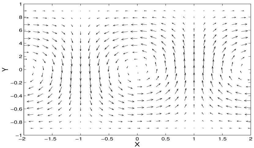
Figure 1: Velocity field: ${\bf v}=\nabla\psi{\times}\hat{{\bf e}}_{z}$ using $\psi$ from (4) with $k=\pi/2$, $\lambda=2.6424$ and $A_{k\lambda}=.3499$

We illustrate, in figure 1, an arrow plot of the velocity field given by choosing $k=\pi/2$, $\lambda=2.6424$ and $A_{k\lambda}=.3499$, in units of $a=1$. The two pressures resulting from the satisfaction of the normal and tangential components of (3) can best be compared by comparing their respective values of $\nabla P$, since $P$ itself is indeterminate up to an additive constant in both cases. In figure 2, we display, as an arrow plot, the difference between the pressure gradients associated with the velocity field shown in figure 1. We have rewritten (1)-(3) in dimensionless units for this purpose, with the kinematic viscosity being replaced by the reciprocal of a Reynolds number, which may be defined as $\mbox{\it Re}=(\langle{\bf v}^{2}\rangle/(k^{2}+\lambda^{2}))^{1/2}/\nu$. Here, the angle brackets refer to the mean of ${\bf v}^{2}$ taken over the 2-D box, containing one period in the $x$ direction and from $y=-a$ to $y=a$. The value of Re used to construct figure 2 is $\mbox{\it Re}\ =2293$, with the dimensionless version of $C_{k\lambda}=5000$ in (4). The two pressures are similar but not identical.

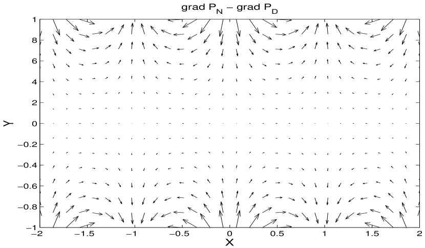
Figure 2: The difference between pressure gradients: $\nabla P_{N}-\nabla P_{D}$ with $\mbox{\it Re}=2293$

In figure 3, a fractional measure of the difference between the “Neumann pressure” $P_{N}$ and the “Dirichlet pressure” $P_{D}$ is exhibited as a contour plot of the scalar ratio

$$\frac{(\nabla P_{D}-\nabla P_{N})^{2}}{\langle(\nabla P_{N})^{2}\rangle}$$ (5)

There is no absolute significance to the numerical value of this ratio. It initially increases with Re  approaching a maximum of about $2\%$ near the wall for $\mbox{\it Re}\mathrel{\hbox to0.0pt{\lower 3.5pt\hbox{$\mathchar 536\relax$}\hss}\raise 2.0pt\hbox{$\mathchar 318\relax$}}10$. It is considered interesting however, that the fractional difference is nearly x-independent where it is largest. That occurs formally because the algebra reveals it to be dominated by a term which varies as $\cosh{(4ky)}-\cos{(4kx)}$ in a region where $ky\mathrel{\hbox to0.0pt{\lower 3.5pt\hbox{$\mathchar 536\relax$}\hss}\raise 2.0pt\hbox{$\mathchar 318\relax$}}1$.

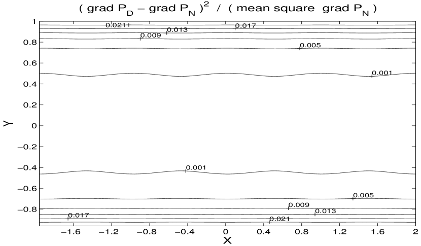
Figure 3: Normalized mean square pressure gradient difference: $(\nabla P_{D}-\nabla P_{N})^{2}/\langle(\nabla P_{N})^{2}\rangle$ with $\mbox{\it Re}=2293$. Note that the fractional difference between the two values of $\nabla P$ is significant only near the wall.

It is amusing but perhaps not significant to superpose the velocity field from (4) with a parabolic plane Poiseuille flow of a larger amplitude. The resulting flow field is shown in figure 4, and it bears a striking but perhaps not significant similarity to the flow patterns seen in two-dimensional plane Poiseuille flow [Jones & Montgomery 1994] when linear stability thresholds are approached. The pressure gradient difference for this case will be fractionally smaller than in figure 3, since pure parabolic plane Poiseuille flow is a rare case where the two pressures happen to agree, and it quantitatively dominates the pressures determined from equation (2) in this example.

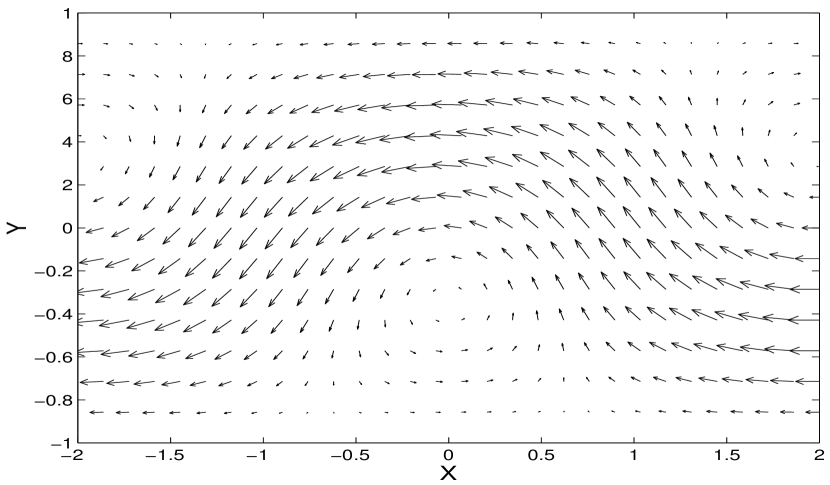
Figure 4: Velocity field shown in figure 1 plus parabolic plane Poiseuille flow: ${\bf v}=\nabla\psi{\times}\hat{{\bf e}}_{z}+2(y^{2}-1)\hat{{\bf e}}_{x}$ with $C_{k\lambda}=1$

3 Discussion and a possible modification

An alternative to the no-slip condition is the “Navier” boundary condition [Lamb 1932]: the slip velocity at the wall surface is taken to be proportional to the rate of shear at the wall. This may be expressed $\Delta V=L_{s}\dot{\gamma}$ where $\Delta V$ is the slip velocity of the fluid at the wall, $\dot{\gamma}$ is the rate of shear at the wall and $L_{s}$ is a constant with the dimensions length. Molecular dynamic simulations of Newtonian liquids under shear [Thompson & Robbins 1990] have shown this to be the case under some circumstances. In fact recent work [Thompson & Troian 1997] has shown that, in cases where the shear rate is large, there is a nonlinear relationship between $L_{s}$ and $\dot{\gamma}$.

We note that the velocity field shown in figure 1 does not lead to one which obeys the Navier boundary condition, after an initial time step, where the fluid has been allowed to slip at the wall. If the velocity field determined by (4) is advanced in time using (1) with the “Neumann pressure”, the proportionality between the slip velocity and the rate of shear at the wall, after the initial time step, varies sinusoidally with $x$.

It is to be stressed that we are concerned here only with initial conditions, not with circumstances under which initial slip velocities might be coaxed dynamically into vanishing after some time.

It is difficult to see in what sense the velocity field obtained from (4) might be an unacceptable one from the point of view of the Navier-Stokes or MHD descriptions. It seems to have all the properties that are thought to be relevant. The family of functions of the same x-periodicity in (4) can be shown to be orthogonal, and is a candidate for a complete set, in which any ${\bf v}$ might be expanded, when supplemented by flux-bearing functions of y alone. The mathematical question of which if any velocity fields, which are both solenoidal and vanish at the wall, would lead to Neumann and Dirichlet pressures that were in agreement with each other, must remain open. Indeed, the question of whether there are any, without some degree of “pre-processing,” must remain open. This is an unsatisfactory situation for fluid mechanics and MHD, in our opinion, even if it is a not unfamiliar one. The search for alternatives seems mandatory.

One alternative that may be explored is one that seemed some time ago, in a rather different context [Shan & Montgomery 1994a,b], to have worked well enough for MHD. Namely, we may think of replacing the requirement of the vanishing of the tangential velocity at a rigid wall with a wall friction term, added to the right hand side of (1), of the form

$$-\frac{\bf v}{\tau({\bf x})}$$ (6)

where the coefficient $1/\tau({\bf x})$ vanishes in the interior of the fluid and rises sharply to a large positive value near the wall. The region over which it is allowed to rise should be smaller than the characteristic thickness of any boundary layer that it might be intended to resolve, but seems otherwise not particularly restrictive. Such a term provides a mechanism for momentum loss to the wall and constrains the tangential velocity to small values, but does not force it to zero. The Dirichlet boundary condition disappears in favor of a relation that permits the time evolution of the tangential components of ${\bf v}$, while demanding that $P$ be determined solely by the Neumann condition (the normal component of (3) only). In a previous MHD application [Shan & Montgomery 1994a,b] dealing with rotating MHD fluids, the scheme seemed to perform acceptably well, but was not intensively tested or benchmarked sharply against any of the better understood Navier-Stokes flows. This comparison seems worthy of future attention.

The work of one of us (D.C.M.) was supported by hospitality in the Fluid Dynamics Laboratory at the Eindhoven University of Technology in the Netherlands. A preliminary account of this work was presented orally at a meeting of the American Physical Society [Kress & Montgomery 1999].

References

- [Batchelor 1967] Batchelor, G. K. 1967 An Introduction to Fluid Mechanics. Cambridge Univ. Press.
- [Canuto et al. 1988] Canuto, C., Hussaini, M.Y., Quarteroni, A. & Zang, T.A. 1988 Spectral Methods in Fluid Mechanics. Springer.
- [Chandrasekhar 1961] Chandrasekhar, S. 1961 Hydrodynamic and Hydromagnetic Stability. Oxford Univ. Press, p.634
- [Gresho 1991] Gresho, P. M. 1991 Incompressible fluid dynamics: some fundamental formulation issues. Annu. Rev. Fluid Mech. 23, 413–453.
- [Kress & Montgomery 1999] Kress, B.T. & Montgomery D.C. 1999 Bull. Am. Phys. Soc. 44, No.8, p.85.
- [Lamb 1932] Lamb, H. 1967 Hydrodynamics. Dover, NY, p.576
- [Roache 1982] Roache, P. J. 1982 Computational Fluid Dynamics. Hermosa Publishers.
- [Jones & Montgomery 1994] Jones, W. B. & Montgomery, D. C. 1994 Finite amplitude steady states of high Reynolds number 2-D channel flow. Physica D 73, 227–243.
- [Shan & Montgomery 1994a] Shan, X. & Montgomery, D.C. 1994a Magnetohydrodynamic stabilization through rotation. Phys. Rev. Letters 73, 1624–1627.
- [Shan & Montgomery 1994b] Shan, X. & Montgomery, D.C. 1994b Rotating magnetohydrodynamics. J. Plasma Physics 52, 113–128.
- [Thompson & Robbins 1990] Thompson, P.A. & Robbins, M.O. 1990 Shear flow near solids: epitaxial order and flow boundary conditions. Phys. Rev.A 41, 6830–6837.
- [Thompson & Troian 1997] Thompson, P.A. & Troian S.M. 1997 A general boundary condition for liquid flow at solid surfaces. Nature 389, 360–362.