Fluid Particle Accelerations in Fully Developed Turbulence

The motion of fluid particles as they are pushed along erratic trajectories by fluctuating pressure gradients is fundamental to transport and mixing in turbulence. It is essential in cloud formation and atmospheric transport[1, 2], processes in stirred chemical reactors and combustion systems[3], and in the industrial production of nanoparticles[4]. The perspective of particle trajectories has been used successfully to describe mixing and transport in turbulence[3, 5], but issues of fundamental importance remain unresolved. One such issue is the Heisenberg-Yaglom prediction of fluid particle accelerations[6, 7], based on the 1941 scaling theory of Kolmogorov[8, 9] (K41). Here we report acceleration measurements using a detector adapted from high-energy physics to track particles in a laboratory water flow at Reynolds numbers up to 63,000. We find that universal K41 scaling of the acceleration variance is attained at high Reynolds numbers. Our data show strong intermittency—particles are observed with accelerations of up to 1,500 times the acceleration of gravity (40 times the root mean square value). Finally, we find that accelerations manifest the anisotropy of the large scale flow at all Reynolds numbers studied.

In principle, fluid particle trajectories are easily measured by seeding a turbulent flow with minute tracer particles and following their motions with an imaging system. In practice this can be a very challenging task since we must fully resolve particle motions which take place on times scales of the order of the Kolmogorov time, $\tau_{\eta}=(\nu/\epsilon)^{1/2}$ where $\nu$ is the kinematic viscosity and $\epsilon$ is the turbulent energy dissipation. This is exemplified in Fig. 1, which shows a measured three-dimensional, time resolved trajectory of a tracer particle undergoing violent accelerations in our turbulent water flow, for which $\tau_{\eta}=0.3\ \mathrm{ms}$. The particle enters the detection volume on the upper right, is pushed to the left by a burst of acceleration and comes nearly to a stop before being rapidly accelerated (1200 times the acceleration of gravity) upward in a cork-screw motion. This trajectory illustrates the difficulty in following tracer particles—a particle’s acceleration can go from zero to 30 times its rms value and back to zero in fractions of a millisecond and within distances of hundreds of micrometers.

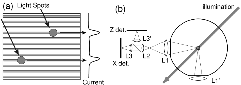
Figure 2: Apparatus (a) Schematic representation of the CLEO III strip detector[12], in which grey bars indicate sense strips which collect charge carriers freed by optical radiation. The 511 strips allow measurement of the one dimensional projection of the light striking the detector. The detector may be read out 70,000 times per second. (b) A combination of lenses (L1, L2, L3, L3’) is used to image the active volume onto a pair of strip detectors which are oriented to measure the $x$ and $y$ coordinates. Another detector assembly may be placed on the opposite port (L1’) to measure $y$ and $z$. The flow is illuminated by a 6 W argon ion laser beam oriented at $45^{\circ}$ with respect to the two viewports. The optics image $(46\pm 7)$ $\mu$m diameter transparent polystyrene spheres which have a density of 1.06 ${\rm g/cm}^{3}$. Particle positions are measured with accuracy 0.1 strips, corresponding to 0.7 $\mu$m in the flow.

Conventional detector technologies are effective for low Reynolds number flows[10, 11], but do not provide adequate temporal resolution at high Reynolds numbers. However, the requirements are met by the use of silicon strip detectors as optical imaging elements in a particle tracking system. The strip detectors employed in our experiment (See Fig. 2a) were developed to measure particle tracks in the vertex detector of the CLEO III experiment operating at the Cornell Electron Positron Collider[12]. When applied to particle tracking in turbulence (See Fig. 2b) each detector measures a one-dimensional projection of the image of the tracer particles. Using a data acquisition system designed for the turbulence experiment, several detectors can be simultaneously read out at up to 70,000 frames per second.

The acceleration of a fluid particle, $\mathbf{a^{+}}$, in a turbulent flow is given by the Navier-Stokes equations,

$$\mathbf{a^{+}}=-\frac{\vec{\nabla}p}{\rho}+\nu\nabla^{2}\mathbf{u}$$ (1)

where $p$ is the pressure, $\rho$ is the fluid density, and $\mathbf{u}$ is the velocity field. In fully developed turbulence the viscous damping term is small compared to the pressure gradient term[13, 14] and therefore the acceleration is closely related to the pressure gradient.

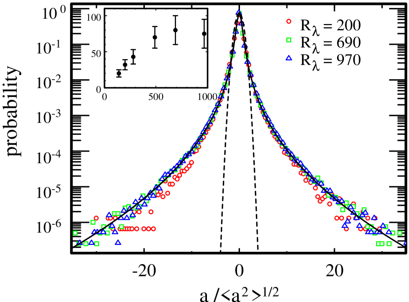
Figure 3: Acceleration Distribution. Probability density functions of the transverse acceleration normalized by its standard deviation at different Reynolds numbers. The acceleration is measured from parabolic fits over $0.75$ $\tau_{\eta}$ segments of each trajectory. The solid line is a parameterization of the highest Reynolds number data using the function $P(a)=C\exp\left(-a^{2}/\left(\left(1+\left|a\beta/\sigma\right|^{\gamma}\right)\sigma^{2}\right)\right)$, with $\beta=0.539$, $\gamma=1.588$, $\sigma=0.508$ and the dashed line is a Gaussian distribution with the same variance. The inset shows the flatness of the acceleration distribution, ($\langle a^{4}\rangle/\langle a^{2}\rangle^{2}$, evaluated using $0.5$ $\tau_{\eta}$ parabolic fits) as a function of $R_{\lambda}$.

Our measurement of the distribution of accelerations is shown in Figure 3, where the probability density function of a normalized acceleration component is plotted at three Reynolds numbers. All of the distributions have a stretched exponential shape, in which the tails extend much further than they would for a Gaussian distribution with the same variance. This indicates that accelerations many times the rms value are not as rare as one might expect, i.e., the acceleration is extremely intermittent. The acceleration flatness, shown in the inset to Fig. 3, characterizes the intermittency of the acceleration, and would be 3 for a Gaussian distribution. These flatness values are consistent with direct numerical simulation (DNS) at low Reynolds number[14] and exceed 60 at the highest Reynolds numbers.

The prediction by Heisenberg and Yaglom for the variance of an acceleration component based on K41 theory is

$$\langle a_{i}a_{j}\rangle=a_{0}\epsilon^{3/2}\nu^{-1/2}\delta_{ij},$$ (2)

where $a_{0}$ is a universal constant which is approximately 1 in a model assuming Gaussian fluctuations[6, 7, 15, 13]. However, DNS has found that $a_{0}$ depends on $\epsilon$. Conventionally this is expressed in terms of the Taylor microscale Reynolds number, $R_{\lambda}$, which is related to the conventional Reynolds number by $R_{\lambda}=(15\mathrm{Re})^{1/2}$ and is proportional to $\epsilon^{1/6}$. Using this notation, DNS results indicate $a_{0}\sim R_{\lambda}^{1/2}$ for $R_{\lambda}<250$[14], with a tendency to level off as $R_{\lambda}$ approaches 470[16].

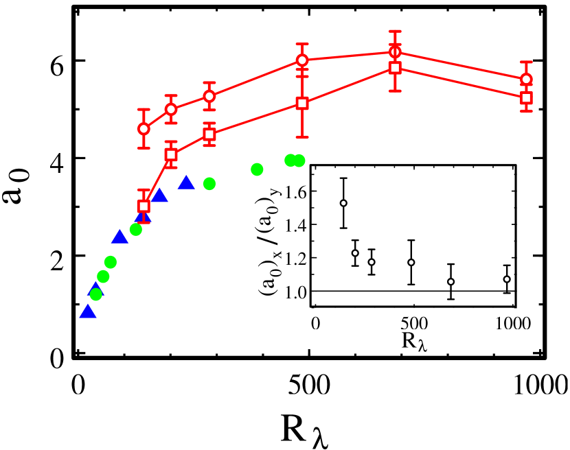
Figure 4: $a_{0}$ as a function of $R_{\lambda}$. Open red circles indicate a transverse component and open red squares the axial component of the acceleration variance. DNS data is represented by blue triangles[14] and green circles[16]. The error bars represent random and systematic errors in the measurement of the acceleration variance. There is an additional uncertainty of 15% in the overall scaling of the vertical axis for the experimental data due to the uncertainty in the measured value of the energy dissipation. The degree to which the 45 $\mu$m diameter tracer particles follow the flow was investigated by measuring the acceleration variance as a function of particle size and density. The results, to be published elsewhere, confirm that the acceleration variance of the $45\mu\mathrm{m}$ particles is within a few percent of the zero particle size limit. The inset shows the ratio of the $a_{0}$ values for transverse and axial components of the acceleration.

Our measurement of the Kolmogorov constant $a_{0}$ is shown in Fig. 4 for eight orders of magnitude of scaling in acceleration variance. We find $a_{0}$ to be anisotropic and to depend significantly on the Reynolds number. The $a_{0}$ values for both components increase as a function of Reynolds number up to $R_{\lambda}\approx 500$, above which they are approximately constant. The trend in $a_{0}$ is consistent with DNS results in the range $140\leq R_{\lambda}\leq 470$[14, 17, 16]. However, the constant value of $a_{0}$ at high Reynolds number suggests that K41 scaling becomes valid at higher Reynolds numbers. Weak deviations from the K41 scaling such as the $a_{0}\sim R_{\lambda}^{0.135}$ prediction of the multifractal model by Borgas[18] cannot be ruled out by our measurements.

The acceleration variance is larger for the transverse component than for the axial component at all values of the Reynolds number. This is shown in the inset to Fig. 4 where the ratio of the Kolmogorov constants for the axial and transverse acceleration components is plotted as a function of Reynolds number. The anisotropy is large at low Reynolds number and diminishes to a small value at $R_{\lambda}=970$. This observation tends to confirm recent experimental results which indicate that anisotropy may persist to much higher Reynolds numbers than previously believed[19, 20].

In summary, our measurements indicate that the Heisenberg-Yaglom scaling of acceleration variance is observed for $500\leq R_{\lambda}\leq 970$. At lower Reynolds number, our measurements are consistent with the anomalous scaling observed in DNS[14, 16]. Our measurements show that the anisotropy of the large scales affects the acceleration components even at $R_{\lambda}\approx 1000$. It is impossible to say on the basis of these measurements if the anisotropy will persist as the Reynolds number approaches infinity. We found the acceleration distribution to be very intermittent, with extremely large accelerations often arising in vortical structures such as the one shown in Fig. 1.

Our results have immediate application for the development of Lagrangian stochastic models, some of which use $a_{0}$ directly as a model constant. These models are being developed and used to efficiently simulate mixing, particulate transport, and combustion in practical flows with varying Reynolds numbers[3, 21, 22]. Our research also has surprising implications for everyday phenomena. For instance, a mosquito flying on a windy day (wind speed 18 km/h and an altitude of 1 meter) would experience an rms acceleration of $15\ \mathrm{m}/\mathrm{s}^{2}$. But given the extremely intermittent nature of the acceleration, our mosquito could expect to experience accelerations of $150\ \mathrm{m}/\mathrm{s}^{2}$ (15 times the acceleration of gravity) every 15 seconds. This may explain why, under windy conditions, a mosquito would prefer to cling to a blade of grass rather than take part in the roller coaster ride through the Earth’s turbulent boundary layer[23].

 

Figure 1: Measured Particle Trajectory The 3-dimensional time-resolved trajectory of a 46 micrometer diameter particle in a turbulent water flow at Reynolds number 63,000 ($R_{\lambda}=970$). A sphere marks the measured position of the particle in each of 300 frames taken every 0.014 ms ($\approx\tau_{\eta}/20$). The shading indicates the acceleration magnitude, with the maximum value of 12,000 m/$\mathrm{s}^{2}$ corresponding to approximately 30 standard deviations. The turbulence is generated between coaxial counter-rotating disks[24, 25] in a closed flow chamber of volume 0.1 $\mathrm{m}^{3}$ with rotation rates ranging from 0.15 Hz to 7.0 Hz, giving rms velocity fluctuation $\tilde{u}$ in the range $0.018\mathrm{m}/\mathrm{s}<\tilde{u}<0.87\mathrm{m}/\mathrm{s}$. Measurements are made in an 8 $\mathrm{mm}^{3}$ volume at the center of the apparatus where the mean velocity is zero and the flow is nearly homogeneous but not isotropic. As a result of a mean stretching of the flow along the propeller axis the rms fluctuations are 1/3 larger for the transverse velocity components than for the axial component. The energy dissipation was determined from measurements of the transverse second order structure function and the Kolmogorov relation $D_{NN}=\frac{4}{3}C_{1}\left(\epsilon r\right)^{2/3}$ with $C_{1}=2.13$[26]. The dissipation was found to be related to the rms velocity fluctuation by $\epsilon={\tilde{u}}^{3}/L$ with an energy injection scale $L=(71\pm 7)\ \mathrm{mm}$. Using the definition of the Taylor microscale Reynolds number $R_{\lambda}=\left(15\tilde{u}L/\nu\right)^{1/2}$ the range of Reynolds numbers accessible is $140\leq R_{\lambda}\leq 970$, (in terms of the classical Reynolds number $1300\leq\mathrm{Re}\leq 63,000$). At the highest Reynolds number the system is characterized by Kolmogorov distance and time scales of $\eta=18\ \mu\mathrm{m}$ and $\tau_{\eta}=0.3\ \mathrm{ms}$, respectively.

References

- [1] Vaillancourt, P. A. and Yau, M. K. Review of particle-turbulence interactions and consequences for cloud physics. B. Am. Meteorol. Soc. 81, 285–298 (2000).
- [2] Weil, J. C., Sykes, R. I., and Venkatram, A. Evaluating air-quality models: Review and outlook. J. Appl. Meteorol. 31, 1121–1145 (1992).
- [3] Pope, S. B. Lagrangian PDF methods for turbulent flows. Annu. Rev. Fluid Mech. 26, 23–63 (1994).
- [4] Pratsinis, Sotiris E., and Srinivas, V. Particle formation in gases, a review. Powder Technol. 88, 267–273 (1996).
- [5] Shraiman, B. I. and Siggia, E. D. Scalar turbulence. Nature 405, 639–646 (2000).
- [6] Heisenberg, W. Zur statistichen theorie der turbulenz. Zschr f. Phys. 124, 628–657 (1948).
- [7] Yaglom, A. M. On the acceleration field in a turbulent flow. C. R. Akad. URSS 67, 795–798 (1949).
- [8] Kolmogorov, A. N. The local structure of turbulence in incompressible viscous fluid for very large Reynolds numbers. Dokl. Akad. Nauk SSSR 30, 301–305 (1941).
- [9] Kolmogorov, A. N. Dissipation of energy in the locally isotropic turbulence. Dokl. Akad. Nauk SSSR 31, 538–540 (1941).
- [10] Virant, M. and Dracos, T. 3D PTV and its application on Lagrangian motion. Meas. Sci. and Technol. 8, 1539–1552 (1997).
- [11] Ott, S. and Mann, J. An experimental investigation of relative diffusion of particle pairs in three-dimensional turbulent flow. J. Fluid Mech. 422, 207–223 (2000).
- [12] Skubic, P., et. al., The CLEO III silicon tracker. Nucl Instrum. Meth. A 418, 40–51 (1998).
- [13] Batchelor, G. K. Pressure fluctuations in isotropic turbulence. Proc. Cambridge Philos. Soc. 47, 359–374 (1951).
- [14] Vedula, P. and Yeung, P. K. Similarity scaling of acceleration and pressure statistics in numerical simulations of isotropic turbulence. Phys. Fluids 11, 1208–1220, (1999).
- [15] Obukhov, A. M. and Yaglom, A. M. The microstructure of turbulent flow. Frikl. Mat. Mekh. 15(3) (1951). translated in National Advisory Committee for Aeronautics (NACA), TM 1350, Washington, DC (1953).
- [16] Gotoh, T. and Fukayama, D. Pressure spectrum in homogeneous turbulence. Submitted to Phys. Rev. Lett. (2000).
- [17] Gotoh, T. and Rogallo, R. S. Intermittancy and scaling of pressure at small scales in forced isotropic turbulence. J. Fluid Mech. 396, 257–285 (1999).
- [18] Borgas, M. S. The multifractal Lagrangian nature of turbulence. Phil. Trans. R. Soc. Lond. A 342(1665), 379–411, (1993).
- [19] Kurien, S. and Sreenivasan, K. R. Anisotropic scaling contributions to high-order structure functions in high-Reynolds-number turbulence. Phys. Rev. E 62, 2206–2212 (2000).
- [20] Shen, X. and Warhaft, Z. The anisotropy of the smale scale structure in high reynolds number () turbulent shear flow. Phys. Fluids 12, 2976–2989 (2000).
- [21] Reynolds, A. M. A second-order Lagrangian stochastic model for particle trajectories in inhomogeneous turbulence. Q. J. R. Meterorol. Soc. 125, 1735–1746 (1999).
- [22] Sawford, B. L. and Yeung, P. K. Eulerian acceleration statistics as a discriminator between Lagrangian stochastic models in uniform shear flow. Phys. Fluids 12, 2033–2045 (2000).
- [23] Bidlingmayer, W. L., Day, J. F., and Evans, D. G. Effect of wind velocity on suction trap catches of some Florida mosquitos. J. Am. Mosquito Contr. 11, 295–301 (1995).
- [24] Voth, G. A., Satyanarayan, K., and Bodenschatz, E. Lagrangian acceleration measurements at large Reynolds numbers. Phys. Fluids 10, 2268–2280 (1998). This paper reports a constant value of at very high Reynolds number. However, our new measurements indicate that the sensor used in this experiment failed to resolve the finest time and length scales of the turbulence because of high noise levels. The correct scaling was obtained, but the numerical values of the acceleration variance and dissipation were inaccurate.
- [25] La Porta, A., Voth, G. A., Moisy, F., and Bodenschatz, E. Using cavitation to measure statistics of low-pressure events in large-Reynolds-number turbulence. Phys. Fluids 12, 1485–1496 (2000).
- [26] Sreenivasan, K. R. On the universality of the Kolmogorov constant. Phys. Fluids 7, 2778–2784 (1995).