Coherent control of enrichment and conversion of
molecular spin isomers

Abstract

A theoretical model of nuclear spin conversion in molecules controlled by an external electromagnetic radiation resonant to rotational transition has been developed. It has been shown that one can produce an enrichment of spin isomers and influence their conversion rates in two ways, through coherences and through level population change induced by radiation. Influence of conversion is ranged from significant speed up to almost complete inhibition of the process by proper choice of frequency and intensity of the external field.

I Introduction

It is well known that many symmetrical molecules exist in Nature only in the form of nuclear spin isomers [1]. Spin isomers are important for fundamental science and have various applications. They can serve as spin labels, influence chemical reactions [2, 3], or tremendously enhance NMR signals [4, 5]. Progress in the spin isomers study depends heavily on available methods for isomer enrichment. Although this field has been significantly advanced recently (see the review in [6]), one needs more efficient enrichment methods.

Recently two enrichment methods based on optically induced change of molecular level populations have been proposed [7, 8]. The purpose of the present paper is to investigate the isomer enrichment caused by optically induced coherences in the molecule.

II Quantum relaxation

Nuclear spin isomers of molecules were discovered in the late 1920s. The most known example is the isomers of H₂. These isomers have different total spin of the two hydrogen nuclei, $I=1$ for ortho molecules and $I=0$ for para molecules. Symmetrical polyatomic molecules have nuclear spin isomers too. For example, CH₃F can be in ortho, or in para state depending on the total spin of three hydrogen nuclei equal 3/2, or 1/2, respectively (see, e.g., [1]). Different spin isomers are often distinguished also by their rotational quantum numbers. Consequently, all rotational states of the molecule are separated into nondegenerate subspaces of different spin states. Schematically, these subspaces for the case of two spin states, ortho and para, are presented in Fig. 1. (For a moment, an optical excitation shown in the ortho space has to be omitted.)

Nuclear spin conversion can be produced by collisions with magnetic particles. This is a well-known mechanism for the conversion of hydrogen imbedded in paramagnetic oxygen [9]. If a molecule is surrounded by nonmagnetic particles, collisions alone cannot change the molecular spin state. In this case the spin conversion is governed by quantum relaxation which can be qualitatively described as follows. Let us split the molecular Hamiltonian into two parts,

$$\hat{H}=\hat{H}_{0}+\hbar\hat{V},$$ (1)

where $\hat{H}_{0}$ is the main term which has the ortho and para states as the eigen states (states in Fig. 1); $\hat{V}$ is a small intramolecular perturbation able to mix the ortho and para states. Suppose that the test molecule was placed initially in the ortho subspace. Due to collisions the molecule starts undergo fast rotational relaxation inside the ortho subspace. This running up and down along the ortho ladder proceeds until the molecule reaches the ortho state $m$ which is mixed with the para state $k$ by the intramolecular perturbation $\hat{V}$. Then, during the free flight just after this collision, the perturbation $\hat{V}$ mixes the para state $k$ with the ortho state $m$. Consequently, the next collision can move the molecule to other para states and thus localize it inside the para subspace. Such mechanism of spin conversion was proposed in the theoretical paper [10] (see also [11]).

Relevance of the described mechanism to actual spin conversion in molecules is not at all obvious. The problem is that the intramolecular perturbations, $\hat{V}$, able to mix ortho and para states are very weak. They have the order of $10-100$ kHz (hyperfine interactions) which should be compared with other much stronger interactions in molecules, or with gas collisions. Nevertheless, the experimental and theoretical proves have been obtained that spin conversion in molecules is indeed governed by quantum relaxation [6, 12, 13, 14]. Although, only three molecules (CH₃F, H₂CO and C₂H₄) have been studied in this context so far, it is very probable that spin conversion in other polyatomic molecules of similar complexity is governed by quantum relaxation too. It is useful for the following to give a few examples of spin conversion rates. Most studied is the spin conversion in ¹³CH₃F which has the rate,

$$\gamma_{13}/P=(12.2\pm 0.6)\cdot 10^{-3}~{}{\text{s}}^{-1}/{\text{Torr}},$$ (2)

in case of pure CH₃F gas [6]. Spin conversion in another isotope modification, ¹²CH₃F, is by almost two orders of magnitude slower [6]. Similar slow conversion was observed in ethylene, ¹³CCH₄, [13],

$$\gamma_{eth}/P=(5.2\pm 0.8)\cdot 10^{-4}~{}{\text{s}}^{-1}/{\text{Torr}}.$$ (3)

These data show that spin conversion by quantum relaxation is on $9-11$ orders of magnitude slower than the rotational relaxation, $\nu\sim 10^{6}-10^{7}$ s^-1/Torr.

III Optical excitation

In this section we will analyze the spin conversion by quantum relaxation in the presence of a resonant electromagnetic radiation. The level scheme is shown in Fig. 1. In order to reveal the main features of the phenomenon we will consider the process in a simplest arrangement. First of all, we assume that molecular states are nondegenerate and that only one ortho-para level pair, $m-k$, is mixed by the intramolecular perturbation, $\hat{V}$. Monochromatic radiation is chosen to be in resonance with the rotational transition $m-n$. In this arrangement the molecular Hamiltonian reads,

$$\hat{H}=\hat{H}_{0}+\hbar\hat{G}+\hbar\hat{V}.$$ (4)

New term, $\hat{G}$, describes the molecular interaction with the radiation,

$$\hat{G}=-({\bf E}_{0}\hat{\bf d}/\hbar)\cos\omega_{L}t,$$ (5)

where ${\bf E}_{0}$ and $\omega_{L}$ are the amplitude and frequency of the electromagnetic wave; $\hat{\bf d}$ is the operator of the molecular electric dipole moment. We have neglected molecular motion in the operator $\hat{G}$ because homogeneous linewidth of pure rotational transition is usually larger than the Doppler width.

Kinetic equation for the density matrix, $\hat{\rho}$, in the representation of the eigen states of the operator $\hat{H}_{0}$ has standard form,

$$d\hat{\rho}/dt={\hat{S}}-i[\hat{G}+\hat{V},\hat{\rho}],$$ (6)

where ${\hat{S}}$ is the collision integral.

Molecules in states ($m,n,k$) interacting with the perturbations $\hat{G}$ and $\hat{V}$ constitute only small fraction of the total concentration of the test molecules. Thus, one can neglect collisions between molecules in these states in comparison with collision with molecules in other states. The latter molecules remain almost at equilibrium. Consequently, the collision integral, ${\hat{S}}$, depends linearly on the density matrix for the disturbed states $m$, $n$, and $k$ even in one component gas. Further, we will assume model of strong collisions for the collision integral. The off-diagonal elements of ${\hat{S}}$ are

$$S_{jj^{\prime}}=-\Gamma\rho_{jj^{\prime}};\ \ \ j,j^{\prime}\in m,n,k;\ \ \ j\neq j^{\prime}.$$ (7)

Here, $j$ and $j^{\prime}$ indicate rotational states of the molecule. The decoherence rates, $\Gamma$, were taken equal for all off-diagonal elements of $\hat{S}$.

Collisions cannot alter molecular spin state in our model. It implies that the diagonal elements of $\hat{S}$ have to be determined separately for ortho molecules,

$$S_{jj}=-\nu\rho_{o}(j)+\nu w_{o}(j)\rho_{o};\ \ \ \rho_{o}=\sum_{j}\rho_{o}(j);\ \ \ j\in{\text{ortho}},$$ (8)

and for para molecules,

$$S_{jj}=-\nu\rho_{p}(j)+\nu w_{p}(j)\rho_{p};\ \ \ \rho_{p}=\sum_{j}\rho_{p}(j);\ \ \ j\in{\text{para}}.$$ (9)

Here $\rho_{o}$, $\rho_{p}$ and $w_{o}(j)$, $w_{p}(j)$ are the total concentrations and Boltzmann distributions of ortho and para molecules. The rotational relaxation rate, $\nu$, was taken equal for ortho and para molecules, because kinetic properties of different spin species are almost identical.

One can obtain from Eq. (6) an equation of change of the total concentration in each spin space [11]. For example, for ortho molecules one has,

$$d\rho_{o}/dt=2Re(i\rho_{mk}V_{km}).$$ (10)

In fact, this result is valid for any model of collision integral as long as collisions do not change the total concentration of molecules in each subspace, i.e., $\sum_{j}S_{jj}=0$ if $j\in$ ortho, or $j\in$ para.

Let us approximate the density matrix by the sum of zero and first order terms over perturbation $\hat{V}$,

$$\hat{\rho}=\hat{\rho}^{(0)}+\hat{\rho}^{(1)}.$$ (11)

In zero order perturbation theory the ortho and para subspaces are independent, i.e., $\rho^{(0)}_{mk}=0$. Consequently, equation of change (10) is reduced to,

$$d\rho_{o}/dt=2Re(i\rho^{(1)}_{mk}V_{km}).$$ (12)

Note that the spin conversion appears in the second order of $\hat{V}$.

Kinetic equations for zero and first order terms of the density matrix are given as,

$$d\hat{\rho}^{(0)}/dt={\hat{S}}^{(0)}-i[\hat{G},\hat{\rho}^{(0)}].$$ (13)

$$d{\hat{\rho}}^{(1)}/dt={\hat{S}}^{(1)}-i[\hat{G},\hat{\rho}^{(1)}]-i[\hat{V},\hat{\rho}^{(0)}].$$ (14)

We start with zero order perturbation theory. In this approximation, the para subspace remain at equilibrium,

$$\rho^{(0)}_{p}(j)=\rho^{(0)}_{p}w_{p}(j);\ \ \ j\in{\text{para}}.$$ (15)

Here $\rho^{(0)}_{p}$ is the total concentration of para molecules.

Density matrix for ortho molecules can be determined from the two equations which follows from Eqs. (7),(8),(13):

$$d\rho^{(0)}_{o}(j)/dt = -\nu\rho^{(0)}_{o}(j)+\nu w_{o}(j)\rho^{(0)}_{o}+2Re(i\rho^{(0)}_{o}(m|n)G_{nm})[\delta_{jm}-\delta_{jn}];$$ (16)

$$d\rho^{(0)}_{o}(m|n)/dt = -\Gamma\rho^{(0)}_{o}(m|n)-iG_{mn}[\rho^{(0)}_{o}(n)-\rho^{(0)}_{o}(m)].$$ (17)

We will assume further the rotational wave approximation,

$$G_{mn}=-Ge^{-i\Omega t};\ \ G\equiv E_{0}\overline{d}_{mn}/2\hbar;\ \ \Omega=\omega_{L}-\omega_{mn},$$ (18)

where the line over symbol indicate a time-independent factor. Rabi frequency, $G$, is assumed to be real. Rotational relaxation, $\nu$, and decoherence, $\Gamma$, are on many orders of magnitude faster than the spin conversion. It allows to assume stationary regime for ortho molecules, thus having, $d\rho^{(0)}_{o}(j)/dt=0$. The substitution, $\rho^{(0)}_{o}(m|n)=\overline{\rho}^{(0)}_{o}(m|n)\exp{(-i\Omega t)}$, transforms Eqs. (17) to algebraic equations which can easily be solved. Thus one has,

$$\rho^{(0)}_{o}(j) = \rho^{(0)}_{o}\left[w_{o}(j)+\frac{2\Gamma}{\nu}\frac{G^{2}\Delta w}{\Gamma^{2}_{B}+\Omega^{2}}(\delta_{jm}-\delta_{jn})\right];$$ (19)

$$\overline{\rho}^{(0)}_{o}(m|n) = \rho^{(0)}_{o}iG\Delta w\frac{\Gamma+i\Omega}{\Gamma^{2}_{B}+\Omega^{2}};$$ (20)

$$\Gamma^{2}_{B} = \Gamma^{2}+4\Gamma G^{2}/\nu;\ \ \ \Delta w\equiv w_{o}(n)-w_{o}(m).$$ (21)

We turn now to the calculation of the first order term, $\rho^{(1)}_{mk}$, which has to be substituted into the equation of change (12). The density matrix element, $\rho^{(1)}_{mk}$, can be found from the two equations which are derived from Eqs. (7),(14),

$$d\rho^{(1)}_{mk}/dt+\Gamma\rho^{(1)}_{mk}+iG_{mn}\rho^{(1)}_{nk} = -iV_{mk}[\rho^{(0)}_{o}(k)-\rho^{(0)}_{o}(m)];$$ (22)

$$d\rho^{(1)}_{nk}/dt+\Gamma\rho^{(1)}_{nk}+iG_{nm}\rho^{(1)}_{mk} = iV_{mk}\rho^{(0)}_{o}(n|m).$$ (23)

Substitution,

$$V_{mk}=\overline{V}e^{i\omega t},\ \ (\omega\equiv\omega_{mk});\ \ \rho^{(1)}_{mk}=\overline{\rho}^{(1)}_{mk}e^{i\omega t};\ \ \rho^{(1)}_{nk}=\overline{\rho}^{(1)}_{nk}e^{i(\omega-\omega_{kn})t},$$ (24)

transforms Eq. (23) to algebraic equations from which one finds $\rho^{(1)}_{mk}$. Then, Eq. (12) gives the following equation for the total concentration of ortho molecules,

$$\frac{d\rho_{o}}{dt}=2|\overline{V}|^{2} Re \frac{[\Gamma+i(\Omega+\omega)][\rho^{(0)}_{p}(k)-\rho^{(0)}_{o}(m)]-iG\overline{\rho}^{(0)}_{o}(n|m)}{F(\Omega)};$$ (25)

$$F(\Omega) \equiv (\Gamma+i\omega)[\Gamma+i(\Omega+\omega)]+G^{2}.$$ (26)

After an appropriate change of notations, the right hand side of Eq. (26), coincides formally with the solution [15] for the work of weak optical field in the presence of strong optical field. Strong field splits the upper state $m$ on two, which appears as two roots of the denominator of Eq. (26) being the second order polynomial on $\omega$. It results in two ortho-para level pairs mixed by the perturbation $\hat{V}$ instead of one pair in the absence of an external field. In analogy with the optical case, one can distinguish the isomer conversion caused by population effects (terms proportional to the level populations $\rho^{(0)}_{p}(k)$ and $\rho^{(0)}_{o}(m)$) and by coherences (term proportional to the off-diagonal density matrix element, $\overline{\rho}^{(0)}_{o}(n|m)$).

Eq. (26) describes time dependence of the concentration of ortho molecules, $\rho_{o}$, in the second order of $\hat{V}$. One can neglect at this approximation small difference between $\rho_{o}$ and $\rho^{(0)}_{o}$. The density of para molecules can be expressed through the density of ortho molecules as, $\rho^{(0)}_{p}=n-\rho^{(0)}_{o}$, where $n$ is the total concentration of the test molecules. Using these points and zero order solution given by Eqs. (15),(21), one can obtain final equation of change for ortho molecules,

$$d\rho_{o}/dt=n\gamma_{op}-\rho_{o}\gamma;\ \ \ \gamma\equiv\gamma_{op}+\gamma_{po}+\gamma_{n}+\gamma_{coh},$$ (27)

where partial conversion rates were introduced,

$$\gamma_{op} = 2|\overline{V}|^{2}w_{p}(k)f(\Omega);\ \ \ \ \ \ \ f(\Omega)\equiv Re\frac{\Gamma+i(\Omega+\omega)}{F(\Omega)};$$ (28)

$$\gamma_{po} = 2|\overline{V}|^{2}w_{o}(m)f(\Omega);$$ (29)

$$\gamma_{n} = 2|\overline{V}|^{2}\frac{G^{2}\Delta w}{\Gamma^{2}_{B}+\Omega^{2}}\frac{2\Gamma}{\nu}f(\Omega);$$ (30)

$$\gamma_{coh} = 2|\overline{V}|^{2}\frac{G^{2}\Delta w}{\Gamma^{2}_{B}+\Omega^{2}}Re\frac{\Gamma-i\Omega}{F(\Omega)}.$$ (31)

Here the rates $\gamma_{op}$, $\gamma_{po}$, and $\gamma_{n}$ are due to molecular level populations and the rate $\gamma_{coh}$ is due to coherences. The terms $\gamma_{op}$ and $\gamma_{po}$ are the only ones which remain in the absence of an external field. In the radiation free case ($G=0$) the result (31) becomes identical with the solution given in [11].

IV Enrichment

Solution to Eq. (27) can be presented as, $\rho_{o}=\overline{\rho}_{o}+\delta\rho_{o}\exp(-\gamma t)$, where time-independent part is given by

$$\overline{\rho}_{o}=n\frac{\gamma_{op}}{\gamma}.$$ (32)

Without an external radiation (at the instant $t=0$), the equilibrium concentration of para molecules is equal to,

$$\rho_{p}(0)=n-\rho_{o}(0)=n\frac{w_{o}(m)}{w_{p}(k)+w_{o}(m)}=\frac{n}{2}.$$ (33)

For simplicity, the Boltzmann factors in Eq. (33) were assumed to be equal, $w_{p}(k)=w_{o}(m)\equiv w$, which implies, $\gamma_{op}=\gamma_{po}$. External field produces a stationary enrichment of para molecules. One can derive from Eqs. (32),(33),

$$\beta\equiv\frac{\overline{\rho}_{p}}{\rho_{p}(0)}-1=1-2\frac{\gamma_{op}}{\gamma}.$$ (34)

An enrichment coefficient, $\beta$, is defined here in such a way that $\beta=0$ if there is no external electromagnetic field. Enrichment of ortho molecules is equal to $-\beta$. Note, that the enrichment, $\beta$, does not depend on the magnitude of intramolecular perturbation $\hat{V}$. It is the consequence of the assumption that only one ortho-para level pair is mixed. Enrichment, $\beta$, depends on the ratio of Boltzmann factors, $w_{o}(n)/w_{o}(m)$, but does not depend on the magnitude of $w_{o}(n)$ itself. In further numerical examples relative difference of the Boltzmann factors will be chosen as $w_{o}(n)=1.2w$.

One needs to specify a few other parameters in order to investigate properties of the optically induced enrichment. We will use, where it is possible, parameters relevant to the spin conversion in ¹³CH₃F. Thus the decoherence rate, $\Gamma$, will be chosen equal 6 MHz, which corresponds to the gas pressure of pure CH₃F equal 0.2 Torr [6]. Rotational relaxation, $\nu$, will be chosen by one order of magnitude slower than the decoherence rate, $\nu=0.1\Gamma$.

Expressions for the enrichment, $\beta$, are given in the Appendix. If ortho-para mixing is performed for a degenerate pair of states $m-k$ ($\omega=0$), the enrichment of para states, $\beta$, has one peak at $\Omega=0$. This peak is determined mainly by population effects.

More interesting is the case of nondegenerate states ($\omega\neq 0$). In this case one has two peaks, at $\Omega=-\omega$ and at $\Omega=0$ (Fig. 2). Peak 1 ($\Omega=-\omega$) is due to the coherent effects determined by $\gamma_{coh}$. Peak 2 ($\Omega=0$) is mainly due to the optically induced level population changes determined by $\gamma_{n}$. In the case of well-separated peaks ($\Gamma_{B}\ll\omega$), the amplitudes of the peak 1 and peak 2 read,

$$A_{1} = \frac{\Delta w}{w}\frac{G^{2}}{\Gamma^{2}+G^{2}}\left[\frac{1}{4}+\frac{D}{\Gamma^{2}_{B}+\omega^{2}}\right];\ \ \ D\equiv\Gamma^{2}+5G^{2}/4-\Gamma G^{2}/\nu+\omega^{2}/4;$$ (35)

$$A_{2} = \frac{\Delta w}{w}\frac{G^{2}}{\Gamma^{2}_{B}}\left[\frac{\Gamma}{\nu}-\frac{3}{4}+\frac{D}{\Gamma^{2}_{B}+G^{2}+\omega^{2}}\right].$$ (36)

Amplitude of the peak 2 grows rapidly with $G$ up to $\beta\simeq 4.5\%$. Amplitude of the peak 1 grows with $G$ to even bigger value $\beta\simeq 5.5\%$. These data are shown in Fig. 3 (upper panel) where points are obtained by fitting an exact expression (34) by two Lorentzians and solid curves are given by Eqs. (36). $\omega$ was chosen equal 130 MHz which corresponds to the ortho-para level gap in ¹³CH₃F [6]. Note, that there is no optically induced enrichment if $\Delta w=0$.

Widths of the enrichment peaks are given by the expressions,

$$W_{1}=2\sqrt{\Gamma^{2}+G^{2}};\ \ \ W_{2}=2\Gamma_{B}.$$ (37)

The two enrichment peaks experience completely different power broadening which are shown in Fig. 3 (low panel). Peak 1 has the width much smaller than the Peak 2. Solid curves in Fig. 3 (low panel) are given by Eqs. (37). Points are obtained by fitting the exact expression for enrichment, $\beta$, by two Lorentzians.

V Conversion

Conversion rate in the presence of an external electromagnetic field has complicated dependence on radiation frequency detuning, $\Omega$, and Rabi frequency, $G$. It is convenient to characterize the conversion rate in relative units,

$$\gamma_{rel}=\frac{\gamma}{\gamma_{free}}-1,$$ (38)

where $\gamma_{free}$ is the field free conversion rate. Similar to the enrichment, $\beta$, this parameter does not depend on magnitude of the perturbation $\hat{V}$ and on absolute values of the Boltzmann factors.

Expressions for the conversion rate, $\gamma_{rel}$, are given in the Appendix. In the case of degenerate ortho-para level pair $m-k$ ($\omega=0$), $\gamma_{rel}$ has narrow negative structure at $\Omega=0$ (Fig. 4). Amplitude of this dip grows rapidly with increasing $G$. If $G\gg\Gamma\gg\nu$, and all Boltzmann factors have the same order of magnitude, the conversion rate at $\Omega=0$ is given by

$$\gamma_{rel}\sim\frac{\Gamma^{2}}{G^{2}}-1.$$ (39)

If $G$ is large, the relative conversion rate, $\gamma_{rel}\simeq-1$, which corresponds to $\gamma\simeq 0$. Thus the spin conversion can be inhibited by radiation having large $G$ and $\Omega=0$.

In the nondegenerate case ($\omega\neq 0$) conversion rate, $\gamma_{rel}$, has two peaks (Fig. 5). If these peaks are well resolved, $\Gamma_{B}\ll\omega^{\prime}$, conversion rate is given by,

$$\gamma_{rel}=\frac{\Gamma^{\prime}\Gamma^{-1}G^{2}}{\Gamma^{\prime 2}+(\Omega+\omega^{\prime})^{2}}+\frac{\Delta w}{w}\frac{G^{2}}{\Gamma^{2}_{B}+\Omega^{2}}\left(\frac{\Gamma}{\nu}-\frac{1}{2}\right),$$ (40)

where new parameters are determined as,

$$\Gamma^{\prime}\equiv\Gamma\left(1+\frac{G^{2}}{\Gamma^{2}+\omega^{2}}\right);\ \ \ \omega^{\prime}\equiv\omega\left(1-\frac{G^{2}}{\Gamma^{2}+\omega^{2}}\right).$$ (41)

The two peaks in the conversion have Lorentzian profiles and amplitudes determined by the expressions,

$$A_{3}=\frac{G^{2}}{\Gamma^{\prime}\Gamma};\ \ \ A_{4}=\frac{\Delta w}{w}\frac{G^{2}}{\Gamma^{2}_{B}}\left(\frac{\Gamma}{\nu}-\frac{1}{2}\right).$$ (42)

These amplitudes are shown in Fig. 6 (upper panel) by solid curves. Points are obtained by fitting the exact solution by two Lorentzians. In this examples, $\omega$ was chosen equal 130 MHz. Peak 4 at $\Omega=0$ is proportional to the ratio of Boltzmann factors. This peak does not grow significantly with $G$. The peak 3 at $\Omega=-\omega^{\prime}$ almost does not depend on Boltzmann factors and at large $G$ grows up to $\gamma_{rel}=(\omega/\Gamma)^{2}$. Thus strong electromagnetic field can speed up the conversion significantly, viz., by two orders of magnitude in our numerical example.

Widths of the two peaks in the conversion rate are determined by the equations,

$$W_{3}=2\Gamma^{\prime};\ \ \ W_{4}=2\Gamma_{B},$$ (43)

and have very different field dependences. In fact, the peak 4 at $\Omega=0$ is broadened even faster than $2\Gamma_{B}$. Peak 3 at $\Omega=-\omega$ has almost no power broadening, if $G\ll\omega$ (Fig. 6, low panel). Solid curves in Fig. 6, low panel, corresponds to the Eqs. (43). Points are obtained by fitting the exact solution by two Lorentzians.

VI Conclusions

We have shown that an external resonant radiation can influence spin isomer conversion in two ways, through level populations and through optically induced coherences. The coherences introduce in the process new and interesting features. In many cases, the coherences play more important role than the level populations. This analysis have been performed in a simplest arrangement in order to reveal the main features of the phenomenon.

Optically induced coherences introduce extra resonances both in enrichment and in conversion frequency dependences. These new resonances are important for future experimental realizations of the optical control of isomer conversion. First, they give convenient opportunity to find coincidences between molecular transitions and available sources of powerful radiation. Second, an observation of the phenomenon will be easier also because electromagnetic radiation can significantly speed up the conversion. Thus steady state enrichment can be achieved much faster than without field. It allows to work at low gas pressures where described above effects can be achieved at smaller radiation intensity.

Another advantage is that one can use resonance at which there is no large radiation absorption and, consequently, no significant level population change by radiation. It should decrease some spurious effects, like molecular resonance exchange. The latter effect can cause serious problems in realization of the optically induced enrichment by population effects [7, 8].

VII Appendix

Here we give expressions for the enrichment, $\beta$, and conversion rate, $\gamma_{rel}$. Enrichment of para molecules is given by Eq. (34). For equal Boltzmann factors, $w_{o}(m)=w_{p}(k)\equiv w$, one has

$$\beta=1-\left(1+\frac{\gamma_{n}+\gamma_{coh}}{2\gamma_{op}}\right)^{-1},$$ (44)

and an approximate expression in case of small enrichment,

$$\beta\simeq\frac{\gamma_{n}+\gamma_{coh}}{2\gamma_{op}}.$$ (45)

Using Eqs. (31), this expression can be reduced to,

$$\beta\simeq \frac{\Delta w}{w} \left[\frac{1/4}{\Gamma^{2}+G^{2}+(\Omega+\omega)^{2}}+\frac{\Gamma/\nu-3/4}{\Gamma^{2}_{B}+\Omega^{2}}+\frac{D}{(\Gamma^{2}_{B}+\Omega^{2})[\Gamma^{2}+G^{2}+(\Omega+\omega)^{2}]}\right];$$ (46)

$$D \equiv \Gamma^{2}+5G^{2}/4-\Gamma G^{2}/\nu+\omega^{2}/4.$$ (47)

There are two peaks in enrichment, at $\Omega=-\omega$ and at $\Omega=0$. These peaks have Lorentzian shape if $\omega\gg\Gamma_{B}$. In the degenerate case ($\omega=0$) there is one peak of complicated form at $\Omega=0$.

The spin conversion rate, $\gamma_{rel}$, is defined as,

$$\gamma_{rel}=\frac{\gamma}{\gamma_{free}}-1.$$ (48)

Using Eqs. (31) one can obtain after straightforward calculations the following expression,

$$\gamma_{rel}= g\frac{(1+g)(\omega^{2}-\Gamma^{2})+2\omega(\Omega+\omega^{\prime})}{\Gamma^{\prime 2}+(\Omega+\omega^{\prime})^{2}}+$$ (52)

$$\frac{\Delta w}{w}\frac{G^{2}}{\Gamma^{2}_{B}+\Omega^{2}}\left(\frac{\Gamma}{\nu}-\frac{1}{2}\right)\left[1+g\frac{(1+g)(\omega^{2}-\Gamma^{2})+2\omega(\Omega+\omega^{\prime})}{\Gamma^{\prime 2}+(\Omega+\omega^{\prime})^{2}}\right]+$$

$$\frac{\Delta w}{2w}\frac{G^{2}}{\Gamma^{2}_{B}+\Omega^{2}}\frac{(1+g)(2\Gamma^{2}+\omega^{2})-\omega(\Omega+\omega^{\prime})}{\Gamma^{\prime 2}+(\Omega+\omega^{\prime})^{2}};$$

$$g\equiv\frac{G^{2}}{\Gamma^{2}+\omega^{2}};\ \ \ \Gamma^{\prime}\equiv\Gamma(1+g);\ \ \ \omega^{\prime}\equiv\omega(1-g).$$

Thus the conversion rate has two peaks situated at $\Omega=-\omega^{\prime}$ and at $\Omega=0$. Position of the peak at $\Omega=\omega^{\prime}$ depends on the field intensity.

In the case of degenerate ortho-para level pair ($\omega=0$), frequency dependence of $\gamma_{rel}$ has complicated shape with a dip in the center at $\Omega=0$ (Fig. (4)). The whole structure is described by the expression,

$$\gamma_{rel}=-\frac{(1+g)G^{2}}{\Gamma^{\prime 2}+\Omega^{2}}+\frac{\Delta w}{w}\frac{G^{2}}{\Gamma^{2}_{B}+\Omega^{2}}\left[\left(\frac{\Gamma}{\nu}-\frac{1}{2}\right)\left(1-\frac{(1+g)G^{2}}{\Gamma^{\prime 2}+\Omega^{2}}\right)+\frac{\Gamma^{\prime}\Gamma}{\Gamma^{\prime 2}+\Omega^{2}}\right].$$ (53)

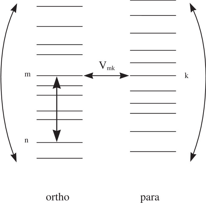
FIG. 1.: Molecular ortho and para states. Bent lines indicate the rotational relaxation. Vertical line shows an optical excitation. $V_{mk}$ gives the ortho-para state mixing by an intramolecular perturbation.

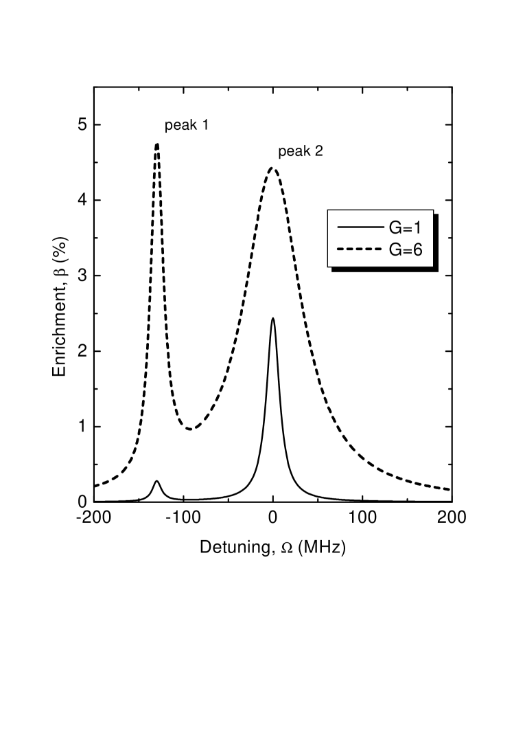
FIG. 2.: Enrichment of para molecules, $\beta$, as a function of radiation frequency detuning, $\Omega$, at $\omega=130$ MHz and two Rabi frequencies, $G=1$ MHz and $G=6$ MHz.

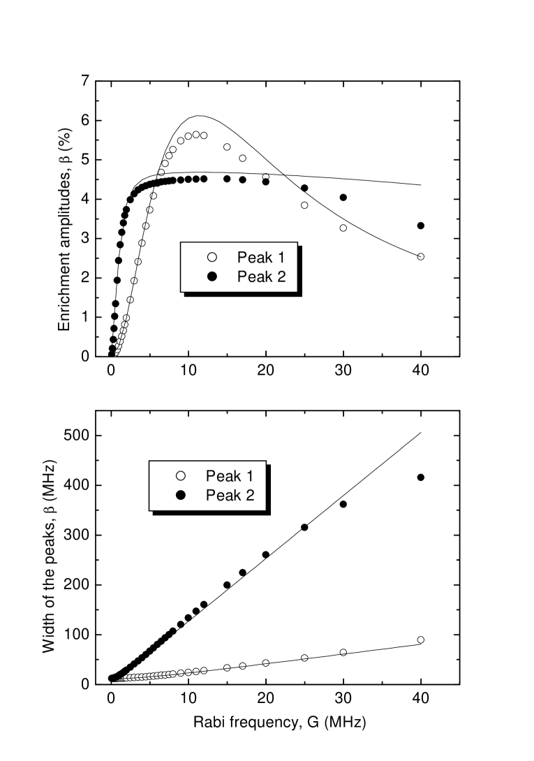
FIG. 3.: Amplitudes of the peaks in enrichment, $\beta$ (upper panel) and width (FWHM) of these peaks (low panel) for the case of $\omega=130$ MHz.

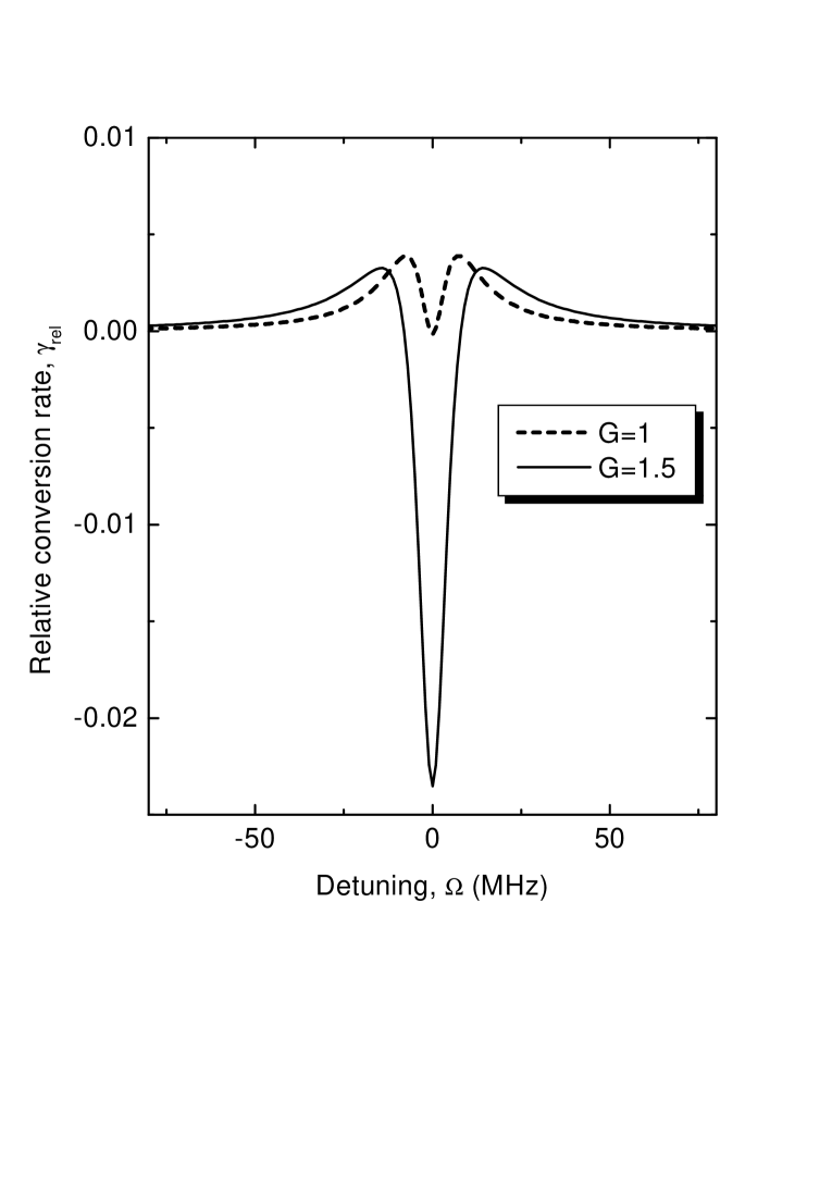
FIG. 4.: Relative conversion rate, $\gamma_{rel}$, for the case of degenerate ortho-para states, $\omega=0$ and the two values of Rabi frequency, $G=1$ MHz and $G=1.5$ MHz.

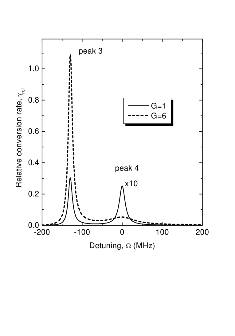
FIG. 5.: Relative conversion rate, $\gamma_{rel}$, for the case of nondegenerate ortho-para states ($\omega=130$ MHz) at two Rabi frequencies, $G=1$ MHz and $G=6$ MHz.

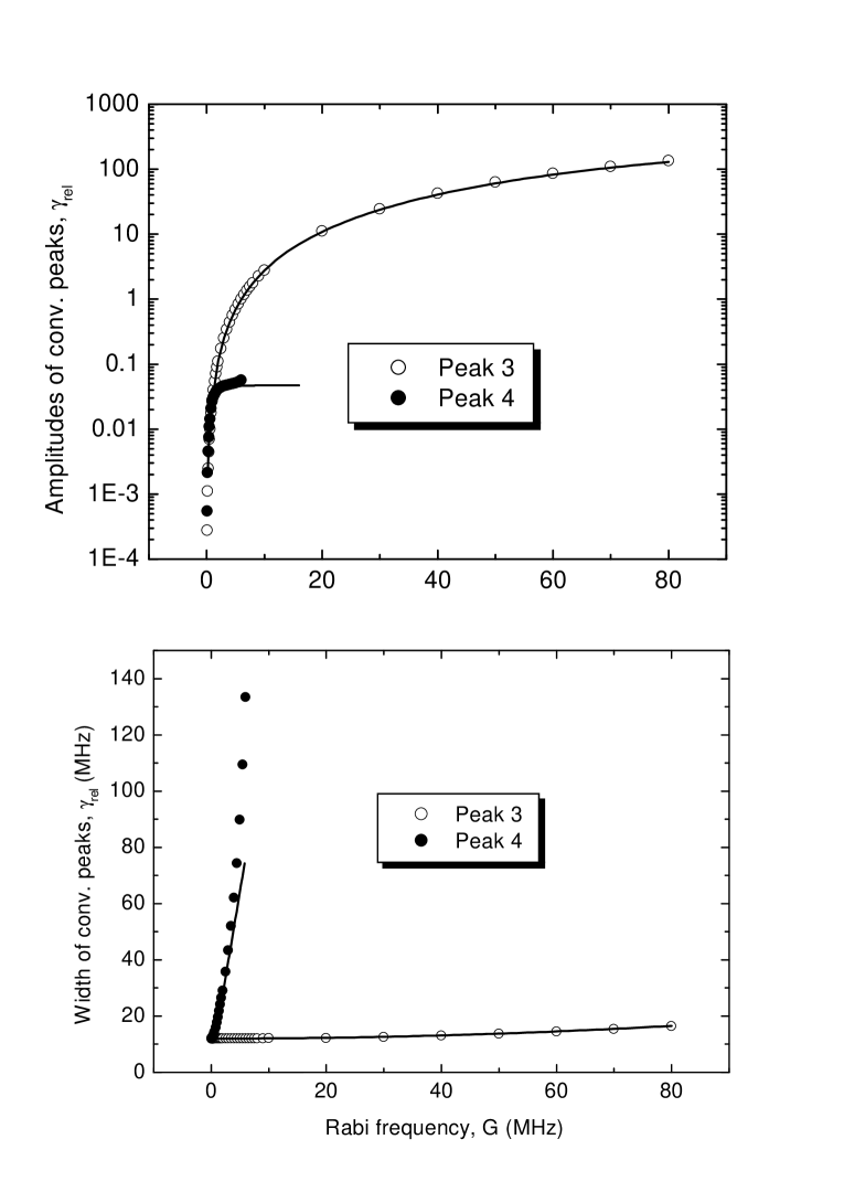
FIG. 6.: Amplitudes of the conversion peaks, $\gamma_{rel}$, (upper panel) and widths (FWHM) of these peaks (low panel) for the nondegenerate case, $\omega=130$ MHz.

REFERENCES

- [1] L. D. Landau and E. M. Lifshitz, Quantum Mechanics, 3rd ed. (Pergamon Press, Oxford, 1981).
- [2] M. Quack, Mol. Phys. 34, 477 (1977).
- [3] D. Uy, M. Cordonnier, and T. Oka, Phys. Rev. Lett. 78, 3844 (1997).
- [4] C. R. Bowers and D. P. Weitekamp, Phys. Rev. Lett. 57, 2645 (1986).
- [5] J. Natterer and J. Bargon, Prog. NUCL. Magn. Reson. Spectr. 31, 293 (1997).
- [6] P. L. Chapovsky and L. J. F. Hermans, Annu. Rev. Phys. Chem. 50, 315 (1999).
- [7] L. V. Il’ichov, L. J. F. Hermans, A. M. Shalagin, and P. L. Chapovsky, Chem. Phys. Lett. 297, 439 (1998).
- [8] A. M. Shalagin and L. V. Il’ichov, Pis’ma Zh. Eksp. Teor. Fiz. 70, 498 (1999).
- [9] E. Wigner, Z. f. Physikal Chemie 23, 28 (1933).
- [10] R. F. Curl, Jr., J. V. V. Kasper, and K. S. Pitzer, J. Chem. Phys. 46, 3220 (1967).
- [11] P. L. Chapovsky, Phys. Rev. A 43, 3624 (1991).
- [12] G. Peters and B. Schramm, Chem. Phys. Lett. 302, 181 (1999).
- [13] P. L. Chapovsky, J. Cosléou, F. Herlemont, M. Khelkhal, and J. Legrand, Chem. Phys. Lett. 322, 414 (2000).
- [14] P. L. Chapovsky and E. Ilisca, (2000), http://arXiv.org/abs/physics/0008083.
- [15] S. G. Rautian, G. I. Smirnov, and A. M. Shalagin, Nonlinear resonances in atom and molecular spectra (Nauka, Siberian Branch, Novosibirsk, Russia, 1979), p. 310.