Wake and Impedance

I Introduction

In this lecture we will develop a concept of wakes and impedances for relativistic beams interacting with the surrounding environment. Among the numerous publications and reviews on this subject, we refer here to recent books chao93 ; zotter98k ; chao99t , where the reader can find a more detailed treatment and further references.

We will use the CGS system of units throughout this paper.

II Interaction of Moving Charges in Free Space

We begin with interactions of particles that moving with constant velocity in free space. If the material walls are far from the particles, their effect in the first approximation can be neglected.

Let us consider a leading particle of charge $q$ moving with velocity $v$, and a trailing particle of unit charge moving behind the leading one on a parallel path at a distance $s$ with an offset $x$, as shown in Fig. 1. We want to find the force which the leading particle exerts on the trailing one.

We will use the following expressions for the electric and magnetic fields of a particle moving with a constant velocity (see, e.g.,landau_lifshitz_ctf ):

$$\textnormal{\boldmath{\hbox{E}}}=\frac{q\textnormal{\boldmath{\hbox{R}}}}{\gamma^{2}R^{*3}}\,,\qquad\textnormal{\boldmath{\hbox{H}}}=\frac{1}{c}\textnormal{\boldmath{\hbox{v}}}\times\textnormal{\boldmath{\hbox{E}}}\,,$$ (1)

where $R$ is the vector drawn from point 1 to point 2, $R^{*2}=s^{2}+x^{2}/\gamma^{2}$, and $\gamma=\left(1-v^{2}/c^{2}\right)^{-1/2}$.

From Eq. (1) we find that the longitudinal force acting on the trailing charge is

$$F_{l}=E_{z}=-\frac{qs}{\gamma^{2}(s^{2}+x^{2}/\gamma^{2})^{3/2}}\,,$$ (2)

and the transverse force is

$$F_{t}=E_{x}-\frac{v}{c}B_{y}=\frac{qx}{\gamma^{4}(s^{2}+x^{2}/\gamma^{2})^{3/2}}\,.$$ (3)

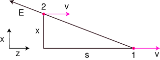
Figure 1: A leading particle 1 and a trailing particle 2 traveling in free space with parallel velocities $v$. Shown also is the coordinate system $x,z$.

In accelerator physics, the force $F$ is often called the space-charge force.

It is easy to see that for any position given by $s$ and $x$, the longitudinal force decreases with the growth of $\gamma$ as $\gamma^{-2}$. For the transverse force, if $s\gg x/\gamma$, $F_{t}\sim\gamma^{-4}$, but for $s=0$, $F_{t}\sim\gamma^{-1}$. Hence, in the limit of ultrarelativistic particles moving parallel to each other, $\gamma\rightarrow\infty$, the electromagnetic interaction in free space vanishes.

In this lecture, we will focus on the case of ultrarelativistic charges, where $v\rightarrow c$. The space-charge effects discussed above disappear in this limit, and the interaction between the particles is due only to the presence of material walls.

Note that, taking the limit $v\rightarrow c$ in Eq. (1) and recalling that $s=vt-z$, we can write the electromagnetic field of an ultrarelitivistic charge in free space as

$$\textnormal{\boldmath{\hbox{E}}}=\frac{2q\textnormal{\boldmath{\hbox{r}}}}{r^{2}}\delta(z-ct)\,,\qquad\textnormal{\boldmath{\hbox{H}}}=\textnormal{\boldmath{\hbox{\hat{z}}}}\times\textnormal{\boldmath{\hbox{E}}}\,,$$ (4)

where $\textnormal{\boldmath$r$}=\textnormal{\boldmath$\hat{x}$}x+\textnormal{\boldmath$\hat{y}$}y$ is a two-dimensional radius vector in a cylindrical coordinate system ($\hat{x}$ and $\hat{y}$ are the unit vectors in the directions of $x$ and $y$, respectively).

III Particles Moving in a Perfectly Conducting Pipe

If particles from the above example move parallel to the axis in a perfectly conducting cylindrical pipe of arbitrary cross section, they induce image charges, on the surface of the wall, that screen the metal from the electromagnetic field of the particles. The image charges travel with the same velocity $v$ (see Fig. 2). Since both the particles and the image charges move on parallel paths, in the limit $v=c$, according to the results in Section II, they do not interact with each other, no matter how close to the wall the particles are.

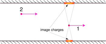
Figure 2: Particles traveling inside a perfectly conducting pipe of arbitrary cross section. Shown are the image charges on the wall generated by the leading charge.

Interaction between the particles in the ultrarelativistic limit can occur if 1) the wall is not perfectly conducting, or 2) the pipe is not cylindrical (which is usually due to the presence of RF cavities, flanges, bellows, beam position monitors, slots, etc., in the vacuum chamber).

IV Causality and the “Catch-Up” Distance

If a beam particle moves along a straight line with the speed of light, the electromagnetic field of this particle scattered off the boundary discontinuities will not overtake it and, furthermore, will not affect the charges that travel ahead of it. The field can interact only with the trailing charges in the beam that move behind it. This constitutes the principle of causality in the theory of wakefields, according to which the interaction of a point charge moving with the speed of light propagates only downstream and never reaches the upstream part of the beam.

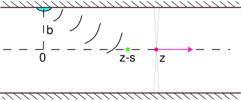
Figure 3: A wall discontinuity located at $z=0$ scatters the electromagnetic field of an ultrarelativistic particle. When the particle moves to location $z$, the scattered field arrives to point $z-s$ .

We can estimate the distance at which the electromagnetic field produced by a leading charge reaches a trailing particles traveling at a distance $s$ behind. Let us assume that a discontinuity located at the surface of a pipe of radius $b$ at coordinate $z=0$ is passed by the leading particle at time $t=0$, see Fig. 3. If the scattered field reaches point $s$ at time $t$, then $ct=\sqrt{(z-s)^{2}+b^{2}}$, where $z$ is a coordinate of the leading particle at time $t$, $z=ct$. Assuming that $s\ll b$, from these two equations we find

$$z\approx\frac{b^{2}}{2s}.$$ (5)

The distance $z$ given by this equation is often called the catch-up distance. Only after the leading charge has traveled this distance away from the discontinuity, can a particle at point $s$ behind it feel the wakefield generated by the discontinuity.

V Round Pipe with Resistive Walls

Consider a round pipe of radius $b$, with finite wall conductivity $\sigma$. A point charge moves along the $z$ axis of the pipe with the speed of light, and a trailing particle follows the leading one at a distance $s$. Both particles are assumed to be on the axis of the pipe. Because of the symmetry of the problem, the only non-zero component of the electromagnetic field on the axis is $E_{z}$, which, depending on the sign, either accelerates or decelerates the trailing charge. Our goal now is to find the field $E_{z}$ as a function of $s$.

If the conductivity of the pipe is large enough, we can use perturbation theory to find the effect of the wall resistivity. In the first approximation, we consider the pipe as a perfectly conducting one. In this case, the electromagnetic field of the charge is the same as in free space and is given by Eqs. (4). For what follows, we will need only the magnetic field $H_{\theta}$,

$$H_{\theta}=\frac{2q}{r}\delta(z-ct).$$ (6)

Using the mathematical identity

$$\delta(z-ct)={1\over 2\pi c}\int_{-\infty}^{\infty}d\omega e^{-i\omega(t-z/c)},$$ (7)

we will decompose $H_{\theta}$ into a Fourier integral,

$$H_{\theta}(r,z,t)=\int_{-\infty}^{\infty}d\omega H_{\theta\omega}(r)e^{-i\omega t+i\omega{z/c}},$$ (8)

where

$$H_{\theta\omega}(r)=\frac{q}{\pi rc}.$$ (9)

In the limit where the skin depth $\delta$ corresponding to the frequency $\omega$, $\delta=c/\sqrt{2\pi\sigma\omega}$, is much smaller than the pipe radius , $\delta\ll b$, we can use the Leontovich boundary condition landau_lifshitz_ecm that relates the tangential electric field $\textnormal{\boldmath$E$}_{t}$ on the wall with the magnetic one,

$$\textnormal{\boldmath{\hbox{E}}}_{t}=\zeta\textnormal{\boldmath{\hbox{H}}}\times\textnormal{\boldmath{\hbox{n}}},$$ (10)

where $n$ is the unit vector normal to the surface and directed toward the metal, and

$$\zeta(\omega)=(1-i)\sqrt{\frac{\omega}{8\pi\sigma}}.$$ (11)

Combining Eqs.(10), (11) and (9), we find

$$E_{z\omega}|_{r=b}=-(1-i)\sqrt{\frac{\omega}{8\pi\sigma}}\frac{q}{\pi bc}.$$ (12)

Equation (12) gives us the longitudinal electric field on the wall, but we need the field on the axis of the pipe. To find the radial dependence of $E_{z\omega}$, we use Maxwell’s equations, from which it follows that the electric field in a vacuum satisfies the wave equation. In the cylindrical coordinate system the wave equation for $E_{z}$ is

$$\frac{1}{c^{2}}\frac{\partial^{2}E_{z}(r,z,t)}{\partial^{2}t}-\Delta E_{z}(r,z,t)$$ (13)

$$= \frac{1}{c^{2}}\frac{\partial^{2}E_{z}(r,z,t)}{\partial^{2}t}-\frac{\partial^{2}E_{z}(r,z,t)}{\partial^{2}z}-\frac{1}{r}\frac{\partial}{\partial r}r\frac{\partial E_{z}(r,z,t)}{\partial r}=0.$$

Substituting the Fourier component $E_{z\omega}(r)e^{-i\omega(t-z/c)}$ into this equation, we find

$$\frac{1}{r}\frac{\partial}{\partial r}r\frac{\partial E_{z\omega}}{\partial r}=0.$$ (14)

This equation has a general solution $E_{z\omega}=A+B\ln r$, where $A$ and $B$ are arbitrary constants. Since we do not expect $E_{z}$ to have a singularity on the axis, $B=0$. Hence the electric field does not depend on $r$, $E_{z\omega}={\rm const}$, and

$$E_{z\omega}|_{r=0}=E_{z\omega}|_{r=b},$$ (15)

implying that $E_{z\omega}|_{r=0}$ is given by the same Eq. (12). Note that we have shown here that in the ultrarelativistic case the longitudinal electric field inside the pipe is constant throughout the pipe cross section.

To find $E_{z}(z,t)$ we make the inverse Fourier transformation,

$$E_{z}(z,t)=\int_{-\infty}^{\infty}d\omega E_{z\omega}e^{-i\omega(t-z/c)},$$ (16)

which gives

$$E_{z}(z,t)=(i-1)\frac{q}{\pi cb}\sqrt{\frac{1}{8\pi\sigma}}\int_{-\infty}^{\infty}d\omega\sqrt{{\omega}}e^{-i\omega(t-z/c)}.$$ (17)

The last integral can be taken analytically in the complex plane (see the Appendix), with the result

$$E_{z}(z,t)={q\over 2\pi b}\sqrt{{c\over\sigma s^{3}}},$$ (18)

for $s>0$. For the points where $s<0$, located in front of the charge, $E_{z}=0$ in agreement with the causality principle. The positive sign of $E_{z}$ indicates that the trailing charge (if it has the same sign as $q$) will be accelerated in the wake.

In our derivation we assumed that the magnetic field on the wall is the same as in the case of perfect conductivity. However, the magnetic field is generated not only by the beam current, but also by a displacement current,

$$j_{z}^{\mathrm{d}isp}={1\over 4\pi}\frac{\partial E_{z}}{\partial t}.$$ (19)

that vanishes in the limit of perfect conductivity. To be able to neglect the corrections to $H_{\theta}$ due to $j_{z}^{\mathrm{d}isp}$, we must require the total displacement current to be much less then the beam current. In the Fourier representation, the time derivative $\partial/\partial t$ reduces to multiplication by $-i\omega$, and the requirement is

$$\pi b^{2}\frac{1}{4\pi}\omega E_{z\omega}\ll I_{\omega}=\frac{q}{2\pi},$$ (20)

or

$$\left({\omega\over c}\right)^{3/2}\ll\sqrt{{4\pi\sigma\over cb^{2}}}.$$ (21)

In the space-time domain, the inverse wavenumber $c/\omega$ corresponds to the distance $s$, and the condition of applicability of Eq. (18) is,

$$s\gg s_{0}=\left({cb^{2}\over 4\pi\sigma}\right)^{1/3}.$$ (22)

The behavior of $E_{z}$ for very small values of $s$, $s<s_{0}$, can be found in Ref. 6.Here we note only that the singularity in Eq. (18) saturates at small $s$, and the electric field changes sign and becomes negative at $s=0$. This field decelerates the leading charge, as expected from the energy balance consideration.

VI Wake Definition

The electromagnetic interaction of charged particles in accelerators with the surrounding environment is usually a relatively small effect that can be considered as a perturbation. In the zeroth approximation, we can assume that the beam moves with a constant velocity along a straight line. We solve Maxwell’s equation, find the fields, and then take into account the effect of these fields on a particle’s motion. In this approach we neglect the second-order effects because the motion along the perturbed orbit can only slightly change the fields computed in the zeroth approximation. Those corrections are usually small, especially for ultrarelativistic particles.

Another important feature of the interaction between the generated electromagnetic field and the particles is that in many cases of practical importance it is localized in a region small compared with the length of the beam orbit. It also occurs on a time scale much smaller than the characteristic oscillation times of the beam in the accelerator (such as betatron and synchrotron periods). This allows us to consider this interaction in the impulse approximation and characterize it by the amount of momentum transferred to the particle.

Taking into account the above considerations, we will introduce the notion of the wake in the following way.

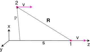
Figure 4: A leading particle 1 and a trailing particle 2 move parallel to each other in a vacuum chamber.

Consider a leading particle 1 of charge $q$ moving along axis $z$ with a velocity close to the speed of light, $v\approx c$, so that $z=ct$ (see Fig. 4). A trailing particle 2 of unit charge moves parallel to the leading one, with the same velocity, at a distance $s$ with offset $\rho$ relative to the $z$-axis. The vector $\rho$ is a two-dimensional vector perpendicular to the $z$-axis, $\textnormal{\boldmath$\rho$}=(x,y)$. Although the two particles move in a vacuum, there are material boundaries in the problem that scatter the electromagnetic field and result in interaction between the particles.

Let us assume that we solved Maxwell’s equation and found the electromagnetic field generated by the first particle. We calculate the change of the momentum $\Delta\textnormal{\boldmath$p$}$ of the second particle caused by this field as a function of the offset $\rho$ and the distance $s$,

$$\Delta\textnormal{\boldmath{\hbox{p}}}(\textnormal{\boldmath{\hbox{\rho}}},s)=\int_{-\infty}^{\infty}dt\left[\textnormal{\boldmath{\hbox{E}}}(\textnormal{\boldmath{\hbox{\rho}}},z,t)+\hat{\textnormal{\boldmath{\hbox{z}}}}\times\textnormal{\boldmath{\hbox{B}}}(\textnormal{\boldmath{\hbox{\rho}}},z,t)\right]_{z=ct-s}\,.$$ (23)

Note that we integrate here along a straight line — the unperturbed orbit of the second particle. The integration limits are extended from minus to plus infinity, assuming that the integral converges.

Since the beam dynamics is different in the longitudinal and transverse directions, it is useful to separate the longitudinal momentum $\Delta p_{z}$ from the transverse component $\Delta\textnormal{\boldmath$p$}_{\perp}$. With the proper sign and the normalization factor $c/q$, these two components are called the longitudinal and transverse wake functions (or simply wakes),

$$w_{l}(\textnormal{\boldmath$\rho$},s) = -\frac{c}{q}\Delta p_{z}=-\frac{c}{q}\int dtE_{z}|_{z=ct-s},$$

$$\textnormal{\boldmath$w$}_{t}(\textnormal{\boldmath$\rho$},s) = \frac{c}{q}\Delta\textnormal{\boldmath$p$}_{\perp}=\frac{c}{q}\int dt\left[\textnormal{\boldmath$E$}_{\perp}+\hat{\textnormal{\boldmath$z$}}\times\textnormal{\boldmath$B$}\right]_{z=ct-s}.$$ (24)

Note the minus sign in the definition of $w_{l}$ — it is introduced so that the positive longitudinal wake corresponds to the energy loss of the trailing particle (if both the leading and trailing particles have the same sign of charge). The defined wakes have dimension ${\rm cm}^{-1}$ in CGS units and V/C in SI units.

Because of the causality principle, the wakefield does not propagate in front of the leading charge, hence

$$w_{l}(\textnormal{\boldmath{\hbox{\rho}}},s)\equiv 0,\qquad\textnormal{\boldmath{\hbox{w}}}_{t}(\textnormal{\boldmath{\hbox{\rho}}},s)\equiv 0,\qquad\mathrm{for}\,\,s<0\,.$$ (25)

It was assumed above that the electromagnetic field is localized in space and time and the integral in Eq. (23) converges. There are cases, however, where this is not true and the source of the wake is distributed uniformly along an extended path, such as the resistive wall wake of a long pipe, considered in Section V. In this case it is more convenient to introduce the wake per unit length of the path by dropping the integration in Eq. (23):

$$w_{l}(\textnormal{\boldmath$\rho$},s) = -\frac{1}{q}E_{z}|_{z=ct-s},$$

$$\textnormal{\boldmath$w$}_{t}(\textnormal{\boldmath$\rho$},s) = \frac{1}{q}\left[\textnormal{\boldmath$E$}_{\perp}+\hat{\textnormal{\boldmath$z$}}\times\textnormal{\boldmath$B$}\right]_{z=ct-s}.$$ (26)

In this definition, the wakes acquire an additional dimension of inverse length, and has the dimension ${\rm cm}^{-2}$ in CGS and V/C/m in SI.

VII Panofsky-Wenzel Theorem

Several general relations between longitudinal and transverse wakes can be obtained from Maxwell’s equation without specifying the boundary condition for the fields.

Let us introduce the vector $\textnormal{\boldmath$R$}=(\textnormal{\boldmath$\rho$},-s)$ (the negative sign in front of $s$ is due to measuring $s$ in the negative direction of $z$, see Fig. 4) and consider momentum $\Delta\textnormal{\boldmath$p$}$ in Eq. (23) as a function of $R$. Let us assume that the electric and magnetic fields are specified through the vector potential $\textnormal{\boldmath$A$}(\textnormal{\boldmath$r$},t)$ and the scalar potential $\phi(\textnormal{\boldmath$r$},t)$, and compute $\Delta\textnormal{\boldmath$p$}$ for the given fields. It is convenient to use the Lagrangian formulation of the equations of motion,

$$\frac{d}{dt}\frac{\partial L}{\partial\textnormal{\boldmath{\hbox{v}}}}=\frac{\partial L}{\partial\textnormal{\boldmath{\hbox{r}}}}\equiv\nabla L,$$ (27)

with the Lagrangian for the trailing unit charge in the electromagnetic field

$$L=-mc^{2}\sqrt{1-\frac{v^{2}}{c^{2}}}+\frac{1}{c}\textnormal{\boldmath{\hbox{A}}}\textnormal{\boldmath{\hbox{v}}}-\phi.$$ (28)

Putting Eq. (28) into Eq. (27) yields ($\textnormal{\boldmath$p$}=m\gamma\textnormal{\boldmath$v$}$)

$$\frac{d}{dt}\left(\textnormal{\boldmath{\hbox{p}}}+\frac{1}{c}\textnormal{\boldmath{\hbox{A}}}\right)=\nabla\left(\frac{1}{c}\textnormal{\boldmath{\hbox{A}}}\textnormal{\boldmath{\hbox{v}}}-\phi\right).$$ (29)

Now, integrating this equation along the orbit of the trailing particle, $x={\rm const}$, $y={\rm const}$ and $z=ct-s$, and assuming that the fields $A$ and $\phi$ vanish at infinity, we find

$$\Delta\textnormal{\boldmath$p$}(\textnormal{\boldmath$R$}) = \int dt\nabla\left(\frac{1}{c}\textnormal{\boldmath$A$}\textnormal{\boldmath$v$}-\phi\right)$$ (30)

$$= \frac{q}{c}\nabla_{\textnormal{\boldmath$R$}}W(\textnormal{\boldmath$R$}),$$

where we introduced the wake potential $W$,

$$W(\textnormal{\boldmath$R$}) = \frac{c}{q}\int dt\left(\frac{1}{c}\textnormal{\boldmath$A$}\textnormal{\boldmath$v$}-\phi\right)$$ (31)

$$= \frac{c}{q}\int dt\left(A_{z}-\phi\right).$$

In the last equation we used $\textnormal{\boldmath$v$}\approx c\hat{\textnormal{\boldmath$z$}}$.

We just proved an important relation that states that all three components of the vector $\Delta\textnormal{\boldmath$p$}$ can be obtained by differentiation of a single scalar function $W$. Recalling now the relation between the components of $\Delta\textnormal{\boldmath$p$}$ and the wakes, Eq. (VI), we find that

$$w_{l}=-\frac{\partial W}{\partial(-s)}=\frac{\partial W}{\partial s},\qquad\textnormal{\boldmath{\hbox{w}}}_{t}=\nabla_{\textnormal{\boldmath{\hbox{\rho}}}}W,$$ (32)

and hence

$${\partial\textnormal{\boldmath{\hbox{w}}}_{t}\over\partial s}=\nabla_{\textnormal{\boldmath{\hbox{\rho}}}}w_{l}.$$ (33)

This relation is usually referred to as the Panofsky-Wenzel theorem. Note that $\nabla_{\textnormal{\boldmath$\rho$}}$ is a two-dimensional gradient with respect to coordinates $x$ and $y$.

One of the most important computational applications of the Panofsky-Wenzel theorem is that knowledge of the longitudinal wake function $w_{l}$ allows us to find the transverse wake $w_{t}$ by means of a simple integration of Eq. (33).

We now prove another important property of $W$: it is a harmonic function of variables $x$ and $y$,

$$\Delta_{\perp}W\equiv\frac{\partial^{2}W}{\partial x^{2}}+\frac{\partial^{2}W}{\partial y^{2}}=0.$$ (34)

To prove this, we will use the fact that both $A$ and $\phi$ satisfy the wave equation in free space, $(\partial^{2}/\partial t^{2}-c^{2}\Delta)\textnormal{\boldmath$A$}=(\partial^{2}/\partial t^{2}-c^{2}\Delta)\phi=0$. Hence

$$0 = \frac{c}{q}\int dt\left(\frac{\partial^{2}}{\partial t^{2}}-c^{2}\Delta\right)\left(A_{z}-\phi\right)$$ (35)

$$= -\frac{c}{q}\int dt\left(\frac{\partial^{2}}{\partial x^{2}}+\frac{\partial^{2}}{\partial y^{2}}\right)\left(A_{z}-\phi\right)+\frac{c}{q}\int dt\left(\frac{\partial^{2}}{\partial t^{2}}-c^{2}\frac{\partial^{2}}{\partial z^{2}}\right)\left(A_{z}-\phi\right)$$

$$= -\frac{\partial^{2}W}{\partial x^{2}}-\frac{\partial^{2}W}{\partial y^{2}}+\frac{c}{q}\int dt\left(\frac{\partial}{\partial t}+c\frac{\partial}{\partial z}\right)\left(\frac{\partial}{\partial t}-c\frac{\partial}{\partial z}\right)\left(A_{z}-\phi\right).$$

The last integral in this equation vanishes because

$$\frac{\partial}{\partial t}+c\frac{\partial}{\partial z}\approx\frac{\partial}{\partial t}+\textnormal{\boldmath{\hbox{v}}}\nabla=\frac{d}{dt}$$ (36)

and

$$\int dt\left(\frac{\partial}{\partial t}+c\frac{\partial}{\partial z}\right)\left(\frac{\partial}{\partial t}-c\frac{\partial}{\partial z}\right)\left(A_{z}-\phi\right)$$ (37)

$$= \int dt\frac{d}{dt}\left(\frac{\partial}{\partial t}-c\frac{\partial}{\partial z}\right)\left(A_{z}-\phi\right)$$

$$= 0.$$

It is interesting that the wake potential $W$ turns out to be a relativistic invariant. A covariant expression for it can be written as

$$W=-\frac{1}{q}\int_{-\infty}^{\infty}A_{k}u^{k}d\tau,$$ (38)

where $A_{k}=(\phi,-\textnormal{\boldmath$A$})$ is the 4-vector potential, $u^{k}=(c\gamma,c\gamma\textnormal{\boldmath$v$})$ is the 4-vector velocity, and $\tau$ is the proper time for the particle.

VIII Systems with a Symmetry Axis

In Section VI we defined the wake as a function of the trailing particle offset relative to the path of the leading particle. In practical applications we are also interested in how the wake depends on the trajectory of the leading particle. We will assume that the system under consideration has a symmetry axis, and choose it as the $z$-axis of the coordinate system (see Fig. 5).

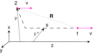
Figure 5: Both the leading particle 1 and the trailing particle 2 are offset relative to the axis of the chamber.

Now the leading particle 1 moves in the $z$ direction with an offset given by vector $\rho^{\prime}$, and the trailing particle travels parallel to the leading one, with the same velocity, at a distance $s$ behind the leading one, and with offset $\rho$ relative to the axis. The vectors $\rho^{\prime}$ and $\rho$ are the two-dimensional vectors perpendicular to the $z$-axis. The wake is still defined by Eq. (VI), but now it will be considered as a function of $\textnormal{\boldmath$\rho$}^{\prime}$, $\rho$, and $s$

$$w_{l} = w_{l}(\textnormal{\boldmath$\rho$},\textnormal{\boldmath$\rho$}^{\prime},s),$$

$$\textnormal{\boldmath$w$}_{t} = \textnormal{\boldmath$w$}_{t}(\textnormal{\boldmath$\rho$},\textnormal{\boldmath$\rho$}^{\prime},s).$$ (39)

Usually the vacuum chamber is designed so that the system axis serves as an ideal orbit for the beam. Deviations from it are relatively small, and both vectors $\rho$ and $\textnormal{\boldmath$\rho$}^{\prime}$ are typically much smaller than the size of the vacuum chamber. We can neglect them in $w_{l}$ and introduce the longitudinal wake function that depends only on $s$,

$$w_{l}(s)=w_{l}(0,0,s).$$ (40)

If the vacuum chamber also has some symmetry elements (e.g., it has either circular, elliptical or rectangular cross section), the transverse wake on the axis, where $\textnormal{\boldmath$\rho$},\textnormal{\boldmath$\rho$}^{\prime}=0$, vanishes, $\textnormal{\boldmath$w$}_{t}(0,0,s)=0$. For small values of $\textnormal{\boldmath$\rho$},\textnormal{\boldmath$\rho$}^{\prime}$ we can expand $\textnormal{\boldmath$w$}_{t}(\textnormal{\boldmath$\rho$},\textnormal{\boldmath$\rho$}^{\prime},s)$ keeping only the lowest-order linear terms. That gives a tensor relation between the transverse wake and the offsets,

$$\textnormal{\boldmath{\hbox{w}}}_{t}(\textnormal{\boldmath{\hbox{\rho}}},\textnormal{\boldmath{\hbox{\rho}}}^{\prime},s)=\overset{\leftrightarrow}{\textnormal{\boldmath{\hbox{W}}}}_{1}(s)\textnormal{\boldmath{\hbox{\rho}}}+\overset{\leftrightarrow}{\textnormal{\boldmath{\hbox{W}}}}_{2}(s)\textnormal{\boldmath{\hbox{\rho'}}},$$ (41)

where $\overset{\leftrightarrow}{\textnormal{\boldmath$W$}}_{1}$ and $\overset{\leftrightarrow}{\textnormal{\boldmath$W$}}_{2}$ are the two-dimensional tensors of rank 2. An example of the wake calculation for elliptical and rectangular cross sections of the pipe can be found in Ref. 7.

IX Axisymmetric Systems

In an axisymmetric system $W$ depends only on the absolute values of $\rho$, $\rho^{\prime}$, and the angle $\theta$ between them. We can always chose a coordinate system such that the vector $\rho^{\prime}$ lies in the $x$-$z$ plane (see Fig. 6), so that the potential function $W$ will be a periodic even function of angle $\theta$ in a cylindrical coordinate system.

Figure 6: Vectors $\rho$ and $\textnormal{\boldmath$\rho$}^{\prime}$ in an axisymmetric system.

Decomposing $W$ in Fourier series in $\theta$ yields

$$W(\rho,\rho^{\prime},\theta,s)=\sum_{m=0}^{\infty}W_{m}(\rho,\rho^{\prime},s)\cos m\theta.$$ (42)

Putting this equation into Eq. (34) gives

$$\sum_{m=0}^{\infty}\left(\frac{1}{\rho}\frac{\partial}{\partial\rho}\rho\frac{\partial W_{m}}{\partial\rho}-\frac{m^{2}}{\rho^{2}}W_{m}\right)\cos m\theta=0,$$ (43)

from which we can find an explicit dependence of $W_{m}$ of $\rho$,

$$W_{m}(\rho,\rho^{\prime},s)=A_{m}(\rho^{\prime},s){\rho}^{m}.$$ (44)

In Eq. (44) we discarded a singular solution of Eq. (43) $W_{m}\propto\rho^{-m}$.

It is also possible to find the dependence of $W_{m}$ versus $\rho^{\prime}$ (see bane85ww ), which turns out to be

$$A_{m}(\rho^{\prime},s)=F_{m}(s)(\rho^{\prime})^{m}.$$ (45)

Using Eq. (32) we now find for the longitudinal and transverse wake functions

$$w_{l}=\sum w_{l}^{(m)},\qquad\textnormal{\boldmath{\hbox{w}}}_{t}=\sum\textnormal{\boldmath{\hbox{w}}}_{t}^{(m)}$$ (46)

where

$$w_{l}^{(m)} = (\rho^{\prime})^{m}\rho^{m}F_{m}^{\prime}(s)\cos m\theta,$$

$$\textnormal{\boldmath$w$}_{t}^{(m)} = m(\rho^{\prime})^{m}\rho^{m-1}F_{m}(s)\left[\hat{\textnormal{\boldmath$r$}}\cos m\theta-\hat{\textnormal{\boldmath$\theta$}}\sin m\theta\right],$$ (47)

where $\hat{\textnormal{\boldmath$r$}}$ and $\hat{\textnormal{\boldmath$\theta$}}$ are the unit vectors in the radial and azimuthal directions in the cylindrical coordinate system. Remember that in this equation we assume that the leading particle is in the plane $\theta=0$.

Equations (IX) are valid for arbitrary values of $\rho$ and $\rho^{\prime}$. Near the axis, where the offsets are small, the higher-order terms with large values of $m$ in these equations also become small. In this case, we can keep only the lower-order terms with $m=0$ (monopole) and $m=1$ (dipole) wakes. For the monopole wake we find

$$w_{l}\equiv w_{l}^{(0)}=F_{0}^{\prime}(s),$$ (48)

which shows that the longitudinal wake does not depend on the radius in an axisymmetric system. We also see that the monopole transverse wake vanishes, $w_{t}^{(0)}=0$.

Since $w_{l}^{(0)}$ does not depend on $\rho^{\prime}$, sometimes it is more convenient to compute the monopole wake for an offset orbit, $\rho^{\prime}\neq 0$, rather than on the axis.

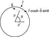
Figure 7: Vectors $\rho$ and $\textnormal{\boldmath$\rho$}^{\prime}$ and unit vectors in cylindrical coordinate system.

For the dipole wake ($m=1$), the vector $\hat{\textnormal{\boldmath$r$}}\cos\theta-\hat{\textnormal{\boldmath$\theta$}}\sin\theta$ lies in the direction of the $x$ axis, that is in the direction of ${\textnormal{\boldmath$\rho$}^{\prime}}$, see Fig. 7. Hence,

$$\textnormal{\boldmath{\hbox{w}}}_{t}^{(1)}={\textnormal{\boldmath{\hbox{\rho}}}^{\prime}}F(s).$$ (49)

The wake given by Eq. (49) is usually normalized by the absolute value of the offset $\rho^{\prime}$, and the scalar function ${w}_{t}^{(1)}/\rho^{\prime}$ is called the transverse dipole wake $w_{t}$,

$$w_{t}(s)=F(s).$$ (50)

Such a transverse wake has the dimension ${\rm cm}^{-2}$ or V/C/m. In this definition, a positive transverse wake means a kick in the direction of the offset of the driving particle (if both particles have the same charge).

X Resistive Wall Wake Functions

We are now in a position to find the wakes generated by a particle in a circular pipe with resistive walls. Using Eq. (18) and the definition Eq. (VI) gives the longitudinal wake

$$w_{l}(s)=-{1\over 2\pi b}\sqrt{{c\over\sigma s^{3}}}\,.$$ (51)

The minus sign here means that the trailing charge is accelerated in the wakefield.

Let us now calculate the dipole transverse wake due to the resistive wall. First, we need to solve for the electromagnetic field of the leading charge $q$ moving with an offset $\textnormal{\boldmath$\rho$}^{\prime}$ in a circular pipe. From the point of view of excitation of dipole modes, this charge can be considered as having a dipole moment $\textnormal{\boldmath$d$}=q\textnormal{\boldmath$\rho$}^{\prime}$. In the zeroth approximation of perturbation theory, the electromagnetic field of a dipole moving with the speed of light in a perfectly conducting pipe is

$$\textnormal{\boldmath{\hbox{E}}}=2\delta(z-ct)\left[\frac{2(\textnormal{\boldmath{\hbox{d}}}\cdot\textnormal{\boldmath{\hbox{r}}})\textnormal{\boldmath{\hbox{r}}}-\textnormal{\boldmath{\hbox{d}}}r^{2}}{r^{4}}+\frac{\textnormal{\boldmath{\hbox{d}}}}{b^{2}}\right]\,,\qquad\textnormal{\boldmath{\hbox{H}}}=\textnormal{\boldmath{\hbox{\hat{z}}}}\times\textnormal{\boldmath{\hbox{E}}}\,.$$ (52)

The first term in the expression for $E$ is a vacuum field of a relativistic dipole, and the second one is due to the image charges, which are generated in order to satisfy the boundary condition on the metal surface.

Following the derivation in Section V, we find the magnetic field on the wall,

$$H_{\theta}=\frac{4d}{b^{2}}\cos\theta\delta(z-ct),$$ (53)

and take its Fourier transform,

$$H_{\theta\omega}=\frac{2d}{\pi cb^{2}}\cos\theta\,,$$ (54)

where the angle $\theta$ is measured from the direction of $d$. Then using the Leontovich boundary condition, Eq. (12), for the electric field $E_{z\omega}$,

$$E_{z\omega}|_{r=b}=-(1-i)\sqrt{\frac{\omega}{8\pi\sigma}}\frac{2d}{\pi cb^{2}}\cos\theta,$$ (55)

and making the inverse Fourier transformation, we obtain $E_{z}$ on the wall

$$E_{z}(z,\rho=b,\rho^{\prime},t)={q\rho^{\prime}\over\pi b^{2}}\sqrt{{c\over\sigma s^{3}}}\cos\theta\,,$$ (56)

where $s=ct-z$. Recalling that, according to Eq. (IX) the dipole wake is a linear function of $\rho$, we conclude that

$$E_{z}(z,\rho,\rho^{\prime},t)={q\rho\rho^{\prime}\over\pi b^{3}}\sqrt{{c\over\sigma s^{3}}}\cos\theta\,,$$ (57)

and the function $F_{1}^{\prime}(s)$ is

$$F_{1}^{\prime}(s)=-{1\over\pi b^{3}}\sqrt{{c\over\sigma s^{3}}}\,,$$ (58)

which gives the following result for the transverse wake defined by Eq. (50):

$$w_{t}(s)={2\over\pi b^{3}}\sqrt{{c\over\sigma s}}\,.$$ (59)

Analogous to the longitudinal wake, Eq. (18), this formula is valid only for $s\gg s_{0}$ (see Eq. (22)).

XI Wakefield in a Bunch of Particles

Up to now we have studied the interaction of two point charges traveling some distance $s$ apart. If a beam consists of $N$ particles with the distribution function $\lambda(s)$ (defined so that $\lambda(s)ds$ gives the probability of finding a particle near point $s$), a given particle will interact with all other particles of the beam. To find the change of the longitudinal momentum of the particle at point $s$ we need to sum the wakes from all other particles in the bunch,

$$\Delta p_{z}(s)=\frac{Ne^{2}}{c}\int_{s}^{\infty}ds^{\prime}\lambda(s^{\prime})w_{l}(s^{\prime}-s).$$ (60)

Here we use the causality principle and integrate only over the part of the bunch ahead of point $s$. In the ultrarelativistic limit the energy change $\Delta E(s)$ caused by the wakefield is equal to $c\Delta p_{z}$, so Eq. (60) can also be rewritten as

$$\Delta E(s)=Ne^{2}\int_{s}^{\infty}ds^{\prime}\lambda(s^{\prime})w_{l}(s^{\prime}-s).$$ (61)

Two integral characteristics of the strength of the wake are the average value of the energy loss $\Delta E_{\mathrm{a}v}$, and the rms spread in energy generated by the wake $\Delta E_{\rm rms}$. These two quantities are defined by the following equations:

$$\Delta E_{\mathrm{a}v}=\int_{-\infty}^{\infty}ds\Delta E(s)\lambda(s),$$ (62)

and

$$\Delta E_{\rm rms}=\left[\int_{-\infty}^{\infty}ds(\Delta E(s)-{\Delta E_{\mathrm{a}v}})^{2}\lambda(s)\right]^{1/2}.$$ (63)

As an example, let us calculate ${\Delta E_{\mathrm{a}v}}$ and $\Delta E_{\rm rms}$ for the resistive wall wake given by Eq. (51) and a Gaussian distribution function,

$$\rho(s)=\frac{1}{\sqrt{2\pi}\sigma_{s}}\exp\left(-\frac{s^{2}}{2\sigma_{s}^{2}}\right),$$ (64)

where $\sigma_{s}$ is the rms bunch length. Note that, since $w$ in Eq. (51) is the wake per unit length of the pipe, we need to multiply the final answer by the pipe length $L$.

A direction substitution of the wake Eq. (51) into Eq. (61) gives a divergent integral when $s^{\prime}\rightarrow s$. To remove the divergence, we need to recall that according to Eq. (48) the longitudinal wake is equal to the derivative of the longitudinal wake potential, $w_{l}=F^{\prime}_{0}(s)$ with $F_{0}=(\pi b)^{-1}\sqrt{c/\sigma s}$ for $s>0$, and $F_{0}=0$ for $s<0$. We then rewrite Eq. (61) as

$$\Delta E(s) = Ne^{2}L\int_{-\infty}^{\infty}ds^{\prime}\lambda(s^{\prime})\frac{dF_{0}(s^{\prime}-s)}{ds}$$ (65)

$$= -Ne^{2}L\int_{s}^{\infty}ds^{\prime}\frac{d\lambda(s^{\prime})}{ds}F_{0}(s^{\prime}-s)$$

$$= {Ne^{2}Lc^{1/2}\over b\sigma_{z}^{3/2}\sigma^{1/2}}G\left(\frac{s}{\sigma_{z}}\right),$$

where the function $G(x)$ is

$$G(x)=\frac{1}{2^{1/2}\pi^{3/2}}\int_{x}^{\infty}\frac{ye^{-y^{2}/2}dy}{\sqrt{y-x}}.$$ (66)

The plot of the function $G\left({s}/{\sigma_{z}}\right)$ is shown in Fig. 8, where the positive values of $s$ correspond to the head of the bunch. We see that in the resistive wake the

Figure 8: Plot of the function $G\left({s}/{\sigma_{z}}\right)$.

particles lose energy in the head of the bunch and get accelerated in the tail. On the average, of course, the losses overcome the gain. For the average energy loss one can find an analytical result:

$$\Delta E_{\mathrm{a}v}={\Gamma({3\over 4})\over 2^{3/2}\pi^{3/2}}{Ne^{2}c^{1/2}\over b\sigma_{z}^{3/2}\sigma^{1/2}}.$$ (67)

Numerical integration of Eq. (63) shows that the energy spread generated by the resistive wake is approximately equal to $\Delta E_{\mathrm{a}v}$:

$$\Delta E_{\rm rms}=1.06\,\Delta E_{\mathrm{a}v}.$$ (68)

If the beam is traveling in the pipe with an offset $y$ relative to the axis, it will be deflected in the direction of the offset, by the transverse wakefields. To calculate the deflection angle $\theta$ we use the relation

$$\theta(s) = \frac{\Delta p_{\perp}(s)}{p}=yL\frac{Ne^{2}}{cp}\int_{s}^{\infty}ds^{\prime}\lambda(s^{\prime})w_{t}(s^{\prime}-s)$$ (69)

$$= {NLr_{e}yc^{1/2}\over\gamma b^{3}\sigma_{z}^{1/2}\sigma^{1/2}}H\left(\frac{s}{\sigma_{z}}\right),$$

where the function $H(x)$ is

$$H(x)=\frac{2^{1/2}}{\pi^{3/2}}\int_{x}^{\infty}\frac{e^{-y^{2}/2}dy}{\sqrt{y-x}}.$$ (70)

The plot of the function $H\left({s}/{\sigma_{z}}\right)$ is shown in Fig. 9.

Figure 9: Plot of the function $H\left({s}/{\sigma_{z}}\right)$.

The deflection angle averaged over the distribution function is

$$\theta_{\mathrm{a}v}={\Gamma({1\over 4})\over 2^{1/2}\pi^{3/2}}{NLr_{e}yc^{1/2}\over\gamma b^{3}\sigma_{z}^{1/2}\sigma^{1/2}},$$ (71)

and the rms spread is

$$\langle(\theta-\theta_{\mathrm{a}v})^{2}\rangle^{1/2}=A^{1/2}{NLr_{e}yc^{1/2}\over\gamma b^{3}\sigma_{z}^{1/2}\sigma^{1/2}},$$ (72)

where

$$A=\frac{2}{\pi^{5/2}}\left[K\left(\frac{3}{4}\right)-\frac{\Gamma^{2}(1/4)}{4\sqrt{\pi}}\right]$$ (73)

and $K$ is the complete elliptic integral. The numerical value of $A^{1/2}$ is 0.186.

XII Definition of Impedance and Relation Between Impedance and Wake

Knowledge of the longitudinal and transverse wake functions gives complete information about the electromagnetic interaction of the beam with its environment. However, in many cases, especially in the study of beam instabilities, it is more convenient to use the Fourier transform of the wake functions, or impedances. Also, it is often easier to calculate the impedance for a given geometry of the beam pipe, rather than the wake function. Recall, that in Section V we actually first computed the Fourier components of the wakes, and then, using the inverse Fourier transformation, found the wakes.

For historical reasons the longitudinal $Z_{l}$ and transverse $Z_{t}$ impedances are defined as Fourier transforms of wakes with different factors,

$$Z_{l}(\omega) = {1\over c}\int_{0}^{\infty}dsw_{l}(s)e^{i\omega s/c}\,,$$

$$Z_{t}(\omega) = -{i\over c}\int_{0}^{\infty}dsw_{t}(s)e^{i\omega s/c}\,.$$ (74)

Note that the integration in Eqs. (XII) can actually be extended into the region of negative values of $s$, because $w_{l}$ and $w_{t}$ are equal to zero in that region.

Impedance can also be defined for complex values of $\omega$ such that ${\rm Im}\omega>0$ and the integrals, Eq. (XII), converge. So defined, the impedance is an analytic function in the upper half-plane of the complex variable $\omega$.

We must keep in mind that other authors sometimes introduce definitions of the impedance that differ from the one given above. In Refs. 2 and 9 the longitudinal impedance is defined as a complex conjugate to the one given by Eq. (XII). Here we follow the definitions of Refs. 1 and 10.

From the definitions in Eq. (XII) it follows that the impedance satisfies the following symmetry conditions:

$${\rm Re}Z_{l}(\omega) = {\rm Re}Z_{l}(-\omega),\qquad\,\,\,\,{\rm Im}Z_{l}(\omega)=-{\rm Im}Z_{l}(-\omega),$$

$${\rm Re}Z_{t}(\omega) = -{\rm Re}Z_{t}(-\omega),\qquad{\rm Im}Z_{t}(\omega)={\rm Im}Z_{t}(-\omega).$$ (75)

The inverse Fourier transform relates the wakes to the impedances:

$$w_{l}(s) = {1\over 2\pi}\int_{-\infty}^{\infty}d\omega Z_{l}(\omega)e^{-i\omega s/c}\,,$$

$$w_{t}(s) = {i\over 2\pi}\int_{\infty}^{\infty}d\omega Z_{t}(\omega)e^{-i\omega s/c}\,.$$ (76)

It turns out that the wakefield can actually be found if only the real part of the impedance is known. Indeed, we can rewrite Eq. (XII) for $w_{l}$ as

$$w_{l}(s)={1\over 2\pi}\int_{\infty}^{\infty}d\omega\left[{\rm Re}Z_{l}(\omega)\cos\frac{\omega s}{c}-{\rm Im}Z_{l}(\omega)\sin\frac{\omega s}{c}\right]\,.$$ (77)

For negative values of $s$ this formula should give $w_{l}=0$, hence

$$0=\int_{\infty}^{\infty}d\omega\left[{\rm Re}Z_{l}(\omega)\cos\frac{\omega s}{c}+{\rm Im}Z_{l}(\omega)\sin\frac{\omega|s|}{c}\right],$$ (78)

from which it follows that

$$w_{l}(s)={1\over\pi}\int_{\infty}^{\infty}d\omega{\rm Re}Z_{l}(\omega)\cos\frac{\omega s}{c}={2\over\pi}\int_{0}^{\infty}d\omega{\rm Re}Z_{l}(\omega)\cos\frac{\omega s}{c}\,.$$ (79)

A similar derivation for the transverse wake gives

$$w_{t}(s)={2\over\pi}\int_{0}^{\infty}d\omega{\rm Re}Z_{t}(\omega)\sin\frac{\omega s}{c}\,.$$ (80)

XIII Energy Loss and ${\rm Re}Z_{l}$

We can relate the energy loss by the bunch to the real part of the longitudinal impedance. Indeed,

$$\Delta E_{\mathrm{a}v} = N^{2}e^{2}\int_{-\infty}^{\infty}ds\lambda(s)\int_{-\infty}^{\infty}ds^{\prime}\lambda(s^{\prime})w_{l}(s^{\prime}-s)$$ (81)

$$= N^{2}e^{2}\int_{-\infty}^{\infty}ds\lambda(s)\int_{-\infty}^{\infty}ds^{\prime}\lambda(s^{\prime})\frac{1}{2\pi}\int_{-\infty}^{\infty}d\omega Z_{l}(\omega)e^{-i\omega(s^{\prime}-s)/c}$$

$$= \frac{N^{2}e^{2}}{2\pi}\int_{-\infty}^{\infty}d\omega Z_{l}(\omega)|\hat{\lambda}(\omega)|^{2},$$

where $\hat{\lambda}(\omega)=\int_{-\infty}^{\infty}ds\lambda(s)e^{i\omega s/c}$. Since $\hat{\lambda}(-\omega)=\hat{\lambda}^{*}(\omega)$, $|\hat{\lambda}(\omega)|^{2}$ is an even function of $\omega$, and

$$\Delta E_{\mathrm{a}v}=\frac{Q^{2}}{\pi}\int_{0}^{\infty}d\omega{\rm Re}Z_{l}(\omega)|\hat{\lambda}(\omega)|^{2},$$ (82)

where $Q=Ne$.

For a point charge, $\lambda(s)=\delta(s)$, $\hat{\lambda}(\omega)=1$, and the energy loss is

$$\Delta E_{\mathrm{a}v}=\frac{e^{2}}{\pi}\int_{0}^{\infty}d\omega{\rm Re}Z_{l}(\omega).$$ (83)

XIV Kramers-Kronig Relations

Equations (79) and (80) relate ${\rm Re}Z(\omega)$ to the wake function. Since $Z(\omega)$ is given by Fourier transformation of $w(s)$, the knowledge of ${\rm Re}Z(\omega)$ allows us to find $Z(\omega)$, and hence ${\rm Im}Z(\omega)$. This means that ${\rm Im}Z(\omega)$ and ${\rm Re}Z(\omega)$ are functionally related to each other. Mathematically this relation is manifested in the Kramers-Kronig dispersion relation, which can be written as

$$Z(\omega)=-\frac{i}{\pi}{\rm P.V.}\int_{-\infty}^{\infty}{Z(\omega^{\prime})\over\omega^{\prime}-\omega}d\omega^{\prime},$$ (84)

where P.V. stands for the principal value of the integral. Taking the real and imaginary parts of this equation gives explicit relations between ${\rm Re}Z$ and ${\rm Im}Z$:

$${\rm Re}Z(\omega) = \frac{1}{\pi}{\rm P.V.}\int_{-\infty}^{\infty}{{\rm Im}Z(\omega^{\prime})\over\omega^{\prime}-\omega}d\omega^{\prime},$$

$${\rm Im}Z(\omega) = -\frac{1}{\pi}{\rm P.V.}\int_{-\infty}^{\infty}{{\rm Re}Z(\omega^{\prime})\over\omega^{\prime}-\omega}d\omega^{\prime}.$$ (85)

XV Useful Formula for Impedance Calculation

Assume that we have a solution of an electromagnetic problem corresponding to the current on the axis of a pipe with the time and space dependence given by $e^{-i\omega t+i\omega{z/c}}$. Specifically, we know the electric field on the axis, $E_{z\omega}(z)e^{-i\omega t}$. How can longitudinal impedance be found in terms of $E_{z\omega}(z)$?

The longitudinal wake is equal to the integrated field $E_{z}$ generated by a point charge moving with the speed of light. The current corresponding to this point charge can be decomposed into a Fourier integral:

$$cq\delta(z-ct)=\int_{-\infty}^{\infty}d\omega{q\over 2\pi}e^{-i\omega(t-z/c)}.$$ (86)

Since we know the electric field generated by each harmonic, we can find the field due to the point charge as a superposition of $E_{z\omega}$:

$$E_{z}(z,t)={q\over 2\pi}\int_{-\infty}^{\infty}d\omega E_{z\omega}(z)e^{-i\omega t}.$$ (87)

For $w_{l}$ we then have

$$w_{l}(s) = -\frac{1}{2\pi}\int_{-\infty}^{\infty}d\omega d(ct)E_{z\omega}(ct-s)e^{-i\omega t}$$ (88)

$$= -\frac{1}{2\pi}\int_{-\infty}^{\infty}d\omega dzE_{z\omega}(z)e^{-i\omega(z+s)/c}.$$

Comparing Eq. (88) with Eq. (XII) we find

$$Z_{l}(\omega)=-\int_{-\infty}^{\infty}dzE_{\omega}(z)e^{-i\omega z/c}.$$ (89)

Hence the longitudinal impedance can be obtained simply by making Fourier transformation of $E_{z\omega}(z)$.

XVI Small Pillbox Cavity in Round Pipe

As an example of using Eq. (89) we will derive here the longitudinal impedance $Z_{l}(\omega)$ for a small axisymmetric cavity (pillbox) in a round perfectly conducting pipe, see Fig. 10. We assume that the wavelength associated with the frequency $\omega$ is much larger than the dimension of the pillbox, $c/\omega\gg g,h$.

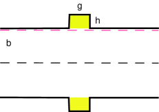
Figure 10: Small pillbox cavity in a round pipe. The dashed line near the wall shows the integration path in Eq. (92).

First, we need to find the solution of Maxwell’s equations corresponding to a unit current $I_{\omega}=e^{-i\omega t+i\omega{z/c}}$ on the axis. Since the cavity is small, the magnitude of the magnetic field at the location of the cavity ($z=0$) is approximately equal to $H_{\theta}$ on the wall of the pipe

$$H_{\theta}=\frac{2}{bc}.$$ (90)

Because $E_{z\omega}$ does not depend on $r$ (see Section V) we can choose the integration path in Eq. (89) close to the wall, as shown in Fig. 10, rather than the pipe axis. Along this path $E_{z\omega}$ is not equal to zero only in the cavity gap, where $|z|\sim h$, and $e^{-i\omega z}\approx 1$. We have

$$Z_{l}(\omega) = -\int_{-\infty}^{\infty}dzE_{z\omega}(z)e^{-i\omega z/c}$$ (91)

$$\approx -\int_{-\infty}^{\infty}dzE_{z\omega}(z)=\frac{1}{c}\frac{d\Phi}{dt}=-\frac{i\omega}{c}\Phi,$$

where $\Phi$ is the magnetic flux in the cross section of the cavity, $\Phi=H_{\theta}hg$. As a result,

$$Z_{l}(\omega)=-i\omega\frac{2gh}{bc^{2}}=-i\omega Z_{0}\frac{gh}{2\pi bc},$$ (92)

where $Z_{0}=4\pi/c=377$ Ohm. What we obtained is a purely inductive longitudinal impedance, which can be rewritten as

$$Z_{l}(\omega)=-i\frac{\omega}{c^{2}}{\cal L},$$ (93)

where the inductance ${\cal L}={2gh}/{b}$. In CGS units the inductance has a dimension of cm, 1 cm = 1 nH.

A more detailed calculation kurennoy94s shows that our method gives only an approximate solution of the problem. In addition to the solenoidal electric field generated by the time-varying magnetic flux in the cavity, there is also a contribution due to the potential component of the electric field. This results in a different numerical coefficient in Eq. (92) which depends on the ratio $g/h$. For example, for $g=h$ the correction factor is 0.84.

XVII Inductive Impedance

We saw in the previous section that a small pillbox is characterized by inductive impedance if the frequency is not very large. This is a common feature of many small perturbations whose size is much smaller than the pipe radius (e.g., small holes, shallow obstacles on the wall, etc.) — for not very large frequencies their impedance is purely inductive.

The longitudinal wake corresponding to the inductive impedance can be found by using Eq. (XII):

$$w_{l}(s)={\cal L}\delta^{\prime}(s).$$ (94)

Because of the inductive wake, slices of the beam can change their energy, although the net energy loss for the bunch is zero because the real part of the impedance vanishes. We can find the energy change as a function of position within the bunch by using Eq. (61). Integration gives

$$\Delta E(s)=-e^{2}N{\cal L}\lambda^{\prime}(s).$$ (95)

For a Gaussian distribution function this reduces to

$$\Delta E(s)={e^{2}N{\cal L}\over\sigma_{z}^{2}}{\xi e^{-\xi^{2}/2}\over\sqrt{2\pi}},$$ (96)

where $\xi=s/\sigma_{z}$. For the rms energy spread we find

$$\langle\Delta E^{2}\rangle^{1/2}={3^{-3/4}(2\pi)^{-1/2}}{e^{2}N{\cal L}\over\sigma_{z}^{2}}.$$ (97)

XVIII Cavity Impedance

In the more general case of a large cavity (Fig. 11) the beam excites cavity eigenmodes and

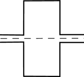
Figure 11: An RF cavity with beam pipes.

the longitudinal wake in the cavity is composed of contributions from single modes,

$$w_{l}(s)=\sum_{n}w^{(n)}(s).$$ (98)

For perfectly conducting walls, assuming that the modes do not propagate into the beam pipes, the mode frequencies $\omega_{n}$ are real. It should be no surprise that each partial wakefield oscillates with the frequency of the mode $\omega_{n}$,

$$w^{(n)}(s)=2k_{n}\cos\left({\omega_{n}s\over c}\right),$$ (99)

where $k_{n}$ is the loss factor, which depends on the geometry of the cavity and the mode number. As an example, for a cylindrical cavity with $b=l$ and $\mathrm{TM}_{010}$ mode, $k_{010}=4.5/l$. For a more rigorous derivation of the wake for a cavity, see Ref. 12.

The cavity impedance for this wake can be calculated by using Eqs. (XII). They give

$${\rm Re}Z_{l} = \pi k_{n}[\delta(\omega+\omega_{n})+\delta(\omega-\omega_{n})],$$

$${\rm Im}Z_{l} = k_{n}\left[\frac{1}{\omega+\omega_{n}}+\frac{1}{\omega-\omega_{n}}\right].$$ (100)

It is also easy to generalize the above wake for a cavity with lossy walls when the frequency of the mode has a small imaginary part $\gamma_{n}$, $\gamma_{n}\ll\omega_{n}$. The wake now decays with time as

$$w_{l}(s)=2k_{n}e^{-\gamma s/c}\cos\left({\omega_{n}s\over c}\right).$$ (101)

Again using Eq. (XII), we can calculate the impedance. It has two peaks: one in the vicinity of $\omega=\omega_{n}$ and the other in the vicinity of $\omega=-\omega_{n}$. Assuming that $\omega$ is close to $\omega_{n}$, we find

$$Z_{l}={k_{n}\over{\gamma-i\left(\omega-\omega_{n}\right)}}.$$ (102)

APPENDIX

We show here how to calculate the integral in Eq. (17),

$$I(\xi)=\int_{-\infty}^{\infty}d\omega\sqrt{\omega}e^{-i\omega\xi},$$ (A1)

where $\xi=t-z/c=s/c$. First, we change the integration variable $\omega$ to $\zeta=\omega\xi$,

$$I(\xi)=\frac{1}{\xi^{3/2}}\int_{-\infty}^{\infty}d\zeta\sqrt{\zeta}e^{-i\zeta}.$$ (A2)

We then consider $\zeta$ as a complex variable. In order to make the integrand a single-valued function in the complex plane, we make a cut along the negative imaginary half-axis and deform the integration path from a straight line to a contour, shown in Fig. 12.

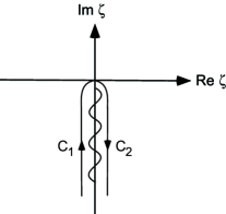
Figure 12: Complex plane $\zeta$. The wavy line indicates the cut. The deformed integration contour consists of two paths, $C_{1}$ and $C_{2}$, corresponding to the integrals $I_{1}$ and $I_{2}$, respectively.

The integral $I(\xi)$ can now be split into two parts, $I_{1}(\xi)$ and $I_{2}(\xi)$, corresponding to the left and right branches of the integration contour.

In the first integral $I_{1}(\xi)$ we change the complex integration variable $\zeta$ to the real positive variable $\tau$, $\zeta=e^{3\pi i/2}\tau=-i\tau$, so that $\sqrt{\zeta}=e^{3\pi i/4}\sqrt{\tau}=(i-1)\sqrt{\tau}/\sqrt{2}$. This gives for $I_{1}$

$$I_{1}(\xi) = \frac{1}{\xi^{3/2}}\int_{\infty}^{0}(-id\tau)\frac{(i-1)\sqrt{\tau}}{\sqrt{2}}e^{-\tau}$$ (A3)

$$= \frac{(i+1)}{\sqrt{2}\xi^{3/2}}\int_{\infty}^{0}d\tau\sqrt{\tau}e^{-\tau}$$

$$= -\frac{\sqrt{\pi}(i+1)}{2^{3/2}\xi^{3/2}}.$$

For the second integral $I_{2}(\xi)$ we choose the real positive variable $\tau$ such that $\zeta=e^{-\pi i/2}\tau=-i\tau$, which means that $\sqrt{\zeta}=e^{-\pi i/4}\sqrt{\tau}=(1-i)\sqrt{\tau}/\sqrt{2}$ and

$$I_{2}(\xi) = \frac{1}{\xi^{3/2}}\int_{0}^{\infty}(-id\tau)\frac{(1-i)\sqrt{\tau}}{\sqrt{2}}e^{-\tau}$$ (A4)

$$= I_{1}(\xi).$$

Hence

$$I(\xi)=I_{1}(\xi)+I_{2}(\xi)=-\frac{\sqrt{\pi}(i+1)}{2^{1/2}\xi^{3/2}}.$$ (A5)

Substituting this equation into Eq. (17) gives Eq. (18).

References

- (1) A. W. Chao, Physics of Collective Beam Instabilities in High Energy Accelerators (Wiley, New York, 1993).
- (2) B. W. Zotter and S. A. Kheifets, Impedances and Wakes in High-Energy Particle Accelerators (World Scientific, Singapore, 1998).
- (3) A. W. Chao and M. Tigner, Handbook of Accelerator Physics and Engineering (World Scientific, Singapore, 1999).
- (4) L. D. Landau and E. M. Lifshitz, The Classical Theory of Fields, vol. 2 of Course of Theoretical Physics, 4th ed. (Pergamon, London, 1979) (Translated from the Russian).
- (5) L. D. Landau and E. M. Lifshitz, Electrodynamics of Continuous Media, vol. 8 of Course of Theoretical Physics, 2nd ed. (Pergamon, London, 1960) (Translated from the Russian).
- (6) K. L. F. Bane and M. Sands, The Short-Range Resistive Wall Wakefields, Tech. Rep. SLAC-PUB-95-7074, SLAC (December 1995).
- (7) R. L. Gluckstern, J. van Zeijts, and B. Zotter, Phys. Rev. E47, 656 (1993).
- (8) K. L. Bane, P. B. Wilson, and T. Weiland, in Proc. US Particle Accelerator School: Physics of Particle Accelerators, Upton, N.Y., 1983 (American Institute of Physics, New York, 1985), no. 127 in AIP Conference Proceedings, pp. 875–928.
- (9) P. B. Wilson, in M. Month and M. Dienes, eds., Proc. US Particle Accelerator School: Physics of Particle Accelerators, Batavia, 1987 (American Institute of Physics, New York, 1989), no. 184 in AIP Conference Proceedings, pp. 525–564.
- (10) S. A. Heifets and S. A. Kheifets, Review of Modern Physics 63, 631 (1991).
- (11) S. S. Kurennoy and G. V. Stupakov, Particle Accelerators 45, 95 (1994).
- (12) P. Wilson, High Energy Electron Linacs: Applications to Storage Ring RF Systems and Linear Colliders, Tech. Rep. SLAC-AP-2884 (Rev.), SLAC (November 1991).