Abstract

The present work shows that through a suitable change of variables relativistic dynamics can be mapped to light propagation in a non-homogeneous medium. A particle’s trajectory through the modified space-time is thus formally equivalent to a light ray and can be derived from a mechanical equivalent of Fermat’s principle. The similarities between light propagation and mechanics are then extended to quantum mechanics, showing that relativistic quantum mechanics can be derived from a wave equation in modified space-time. Non-relativistic results, such as de Broglie’s wavelength, Schrödinger equation and uncertainty principle are shown to be direct consequences of the theory and it is argued that relativistic conclusions are also possible.

1 Introduction

This paper is presented in a rather crude state; the text is imperfect and some conclusions are deferred to ulterior publications; nevertheless the author feels that this work must be diffused even in a preliminary stage due to its significance. The author’s presence at the OSA’s annual meeting provided an opportunity for the presentation of his work that he could not despise.

The similarities between light propagation and wave mechanics have been pointed out by numerous authors, although a perfect mapping from one system to the other has never been achieved. Almeida et al. [1] showed that near-field light diffraction could be calculated using the Wigner Distribution Function (WDF) and obtained results proving the existence of super-resolution in certain circumstances.

The study of wide angle light propagation makes use of a transformation which brings to mind the Lorentz transformation of special relativity. It was then natural to try an association of Newtonian mechanics to paraxial optics and special relativity to wide angle propagation. This process promoted the definition of a coordinate transformation to render the relativistic space homologous to the optical space. The introduction of a variational principle allowed the derivation of relativistic dynamics in the modified space-time in a process similar to the derivation of optical propagation from Fermat’s principle. One important consequence is that each particle travels through modified space-time with the speed of light.

The similarity could be carried further to diffraction phenomena and quantum mechanics. It was postulated that a particle has an intrinsic frequency related to its mass and many important results were derived directly from this statement. More general results will probably be feasible in the future.

2 Notes on Hamiltonian optics

The propagation of an optical ray is governed by Fermat’s principle, which can be stated [2]:

$$\delta\int_{P_{1}}^{P_{2}}nds=0~{}.$$ (1)

The integral quantity is called point characteristic and measures the optical path length between points $P_{1}$ and $P_{2}$.

$$V(x_{1},y_{1},x_{2},y_{2})=\int_{P_{1}}^{P_{2}}nds~{}.$$ (2)

The quantity $ds$ is the length measured along a ray path and can be replaced by:

$$ds=\frac{dz}{(1-u_{x}^{2}-u_{y}^{2})^{1/2}}=\frac{dz}{u_{z}}~{},$$ (3)

where $u_{x}$, $u_{y}$ and $u_{z}$ are the ray direction cosines with respect to the $x$, $y$ and $z$ axes.

Inserting Eq. (3) into Eq. (1) we have:

$$\delta\int_{z_{1}}^{z_{2}}\frac{ndz}{(1-u_{x}^{2}-u_{y}^{2})^{1/2}}=0~{},$$

$$\delta\int_{z_{1}}^{z_{2}}\frac{ndz}{u_{z}}=0~{}.$$ (4)

Of course we can also write:

$$ds=(1+\dot{x}^{2}+\dot{y}^{2})^{1/2}dz~{},$$ (5)

with

$$\dot{x}=\frac{dx}{dz}~{}~{}\mathrm{and}~{}~{}\dot{y}=\frac{dy}{dz}~{}.$$ (6)

It is easy to relate $\dot{x}$ and $\dot{y}$ to $u_{x}$ and $u_{y}$:

$$u_{x} = \frac{\dot{x}}{(1+\dot{x}^{2}+\dot{y}^{2})^{1/2}}~{},$$

$$u_{y} = \frac{\dot{y}}{(1+\dot{x}^{2}+\dot{y}^{2})^{1/2}}~{},$$ (7)

where only the positive root is considered.

Inserting Eq. (5) into Eq. (1) we get:

$$\delta\int_{z_{1}}^{z_{2}}n(1+\dot{x}^{2}+\dot{y}^{2})^{1/2}dz=0~{}.$$ (8)

We can use the position coordinates $x$ and $y$ as generalized coordinates and $z$ for time, in order to define the Lagrangian. We have [3, 4]:

$$L=n(1+\dot{x}^{2}+\dot{y}^{2})^{1/2}$$ (9)

Euler Lagrange’s propagation equations are:

$$\frac{d}{dz}\frac{\partial L}{\partial\dot{x}}-\frac{\partial L}{\partial x} = 0~{},$$ (10)

$$\frac{d}{dz}\frac{\partial L}{\partial\dot{y}}-\frac{\partial L}{\partial y} = 0~{};$$ (11)

We can go a step further if we define a system Hamiltonian and write the canonical equations; we start by finding the components of the conjugate momentum ($\mathbf{p}$) from the Lagrangian. Knowing that $n$ is a function of $x$, $y$ and $z$, the conjugate momentum components can be written as:

$$p_{x} = \frac{\partial L}{\partial\dot{x}}=\frac{n\dot{x}}{(1+\dot{x}^{2}+\dot{y}^{2})^{1/2}}~{},$$

$$p_{y} = \frac{\partial L}{\partial\dot{y}}=\frac{n\dot{y}}{(1+\dot{x}^{2}+\dot{y}^{2})^{1/2}}~{}.$$ (12)

If we consider Eq. (2), the result is:

$$p_{x} = nu_{x}~{},$$

$$p_{y} = nu_{y}~{}.$$ (13)

The system Hamiltonian is:

$$H = p_{x}\dot{x}+p_{y}\dot{y}-L$$ (14)

$$= \frac{n(\dot{x}^{2}+\dot{y}^{2})}{(1+\dot{x}^{2}+\dot{y}^{2})^{1/2}}-L$$

$$= \frac{-n}{(1+\dot{x}^{2}+\dot{y}^{2})^{1/2}}$$

$$= -n(1-u_{x}^{2}-u_{y}^{2})^{1/2}~{},$$

$$= -nu_{z}~{},$$

The Hamiltonian has the interesting property of having the dependence on the generalized coordinates and time, separated from the dependence on the conjugate momentum. The canonical equations are:

$$\dot{x} = \frac{\partial H}{\partial p_{x}}=\frac{u_{x}}{(1-u_{x}^{2}-u_{y}^{2})^{1/2}}~{}=~{}\frac{u_{x}}{u_{z}}~{},$$

$$\dot{y} = \frac{\partial H}{\partial p_{y}}=\frac{u_{y}}{(1-u_{x}^{2}-u_{y}^{2})^{1/2}}~{}=~{}\frac{u_{y}}{u_{z}}~{},$$

$$n\dot{u}_{x}+\dot{n}u_{x} = -\frac{\partial H}{\partial x}=(1-u_{x}^{2}-u_{y}^{2})^{1/2}\frac{\partial n}{\partial x}~{}=~{}u_{z}\frac{\partial n}{\partial x}~{},$$

$$n\dot{u}_{y}+\dot{n}u_{y} = -\frac{\partial H}{\partial y}=(1-u_{x}^{2}-u_{y}^{2})^{1/2}\frac{\partial n}{\partial y}~{}=~{}u_{z}\frac{\partial n}{\partial y}~{}.$$ (15)

Obviously the first two canonical equations represent just a trigonometric relationship.

It is interesting to note that if the refractive index varies only with $z$, then the conjugate momentum will stay unaltered; the direction cosines will vary accordingly to keep constant the products $nu_{x}$ and $nu_{y}$.

We will now consider an non-homogeneous medium with a direction dependent refractive index and will add this dependence as a correction to a nominal index.

$$n=n_{0}-\frac{n_{c}}{\left(1+\dot{x}^{2}+\dot{y}^{2}\right)^{1/2}},$$ (16)

where $n_{0}$ is the nominal index and $n_{c}$ is a correction parameter. Eq. (9) becomes

$$L=n_{0}\left(1+\dot{x}^{2}+\dot{y}^{2}\right)-n_{c}.$$ (17)

We will follow the procedure for establishing the canonical equations in this new situation. It is clear that the momentum is still given by Eq. (2) if $n$ is replaced by $n_{0}$.

The new Hamiltonian is given by

$$H=-n_{0}(1-u_{x}^{2}-u_{y}^{2})+n_{c},$$ (18)

and the canonical equations become

$$\dot{x} = \frac{\partial H}{\partial p_{x}}=\frac{u_{x}}{(1-u_{x}^{2}-u_{y}^{2})^{1/2}}~{}=~{}\frac{u_{x}}{u_{z}}~{},$$

$$\dot{y} = \frac{\partial H}{\partial p_{y}}=\frac{u_{y}}{(1-u_{x}^{2}-u_{y}^{2})^{1/2}}~{}=~{}\frac{u_{y}}{u_{z}}~{},$$

$$n_{0}\dot{u}_{x}+\dot{n}_{0}u_{x} = -\frac{\partial H}{\partial x}=u_{z}\frac{\partial n_{0}}{\partial x}~{}-\frac{\partial n_{c}}{\partial x}~{},$$

$$n_{0}\dot{u}_{y}+\dot{n}_{0}u_{y} = -\frac{\partial H}{\partial y}=u_{z}\frac{\partial n_{0}}{\partial y}~{}-\frac{\partial n_{c}}{\partial y}~{}.$$ (19)

The present discussion of non-homogeneous media is not completely general but is adequate for highlighting similarities with special relativity and quantum mechanics, as is the purpose of this work.

3 Diffraction and Wigner distribution function

Almeida et al. [1] have shown that the high spatial frequencies in the diffracted spectrum cannot be propagated and this can even, in some cases, lead to a diffraction limit much lower than the wavelength; here we detail those arguments.

The Wigner distribution function (WDF) of a scalar, time harmonic, and coherent field distribution $\varphi(\mathbf{q},z)$ can be defined at a $z=\mathrm{const.}$ plane in terms of either the field distribution or its Fourier transform $\overline{\varphi}(\mathbf{p})=\int\varphi(\mathbf{q})\exp(-ik\mathbf{q}^{T}\mathbf{p})d\mathbf{q}$ [5, 6, 7]:

$$W(\mathbf{q},\mathbf{p}) = \int\varphi\left(\mathbf{q}+\frac{\mathbf{q}^{\prime}}{2}\right)\varphi^{*}\left(\mathbf{q}-\frac{\mathbf{q}^{\prime}}{2}\right)\exp\left(-ik\mathbf{q}^{\prime T}\mathbf{p}\right)d\mathbf{q}^{\prime}$$ (20)

$$= \frac{k^{2}}{4\pi^{2}}\int\overline{\varphi}\left(\mathbf{p}+\frac{\mathbf{p}^{\prime}}{2}\right)\overline{\varphi}^{*}\left(\mathbf{p}-\frac{\mathbf{p}^{\prime}}{2}\right)\exp\left(ik\mathbf{q}^{T}\mathbf{p}^{\prime}\right)d\mathbf{p}^{\prime}~{},$$ (21)

where $k=2\pi/\lambda$, ^∗ indicates complex conjugate and

$$\mathbf{q} = \left(x,y\right),$$ (22)

$$\mathbf{p} = \left(nu_{x},nu_{y}\right).$$ (23)

In the paraxial approximation, propagation in a homogeneous medium of refractive index $n$ transforms the WDF according to the relation

$$W(\mathbf{q},\mathbf{p},z)=W(\mathbf{q}-\frac{z}{n}\mathbf{p},\mathbf{p},0).$$ (24)

After the WDF has been propagated over a distance, the field distribution can be recovered by [6, 7]

$$\varphi(\mathbf{q},z)\varphi^{*}(0,z)=\frac{1}{4\pi^{2}}\int W(\mathbf{q}/2,\mathbf{p},z)\exp(i\mathbf{q}\mathbf{p})d\mathbf{p}.$$ (25)

The field intensity distribution can also be found by

$$|\varphi(\mathbf{q},z)|^{2}=\frac{4\pi^{2}}{k^{2}}\int W(\mathbf{q},\mathbf{p},z)d\mathbf{p}.$$ (26)

Eqs. (25) and (26) are all that is needed for the evaluation of Fresnel diffraction fields. Consider the diffraction pattern for a rectangular aperture in one dimension illuminated by a monocromatic wave propagating in the $z$ direction. The field distribution immediately after the aperture is given by

$$\varphi(x,0)=1~{}~{} \rightarrow ~{}~{}|x|<l/2,$$

$$\varphi(x,0)=0~{}~{} \rightarrow ~{}~{}|x|\geq l/2,$$ (27)

with $l$ being the aperture width.

Considering that $\varphi(x,0)$ is real we can write

$$\varphi\left(x+\frac{x^{\prime}}{2}\right)\varphi^{*}\left(x-\frac{x^{\prime}}{2}\right)=\mathrm{H}\left(\frac{l}{2}+\frac{x^{\prime}}{2}-|x|\right)\mathrm{H}\left(\frac{l}{2}-\frac{x^{\prime}}{2}-|x|\right).$$ (28)

We then apply Eq. (28) to the WDF definition Eq. (20) to find

$$W(x,p_{x})=0~{}~{} \rightarrow ~{}~{}|x|\geq l/2,$$

$$W(x,p_{x})=\frac{2\sin[kp_{x}(l-2x)]}{kp_{x}}~{}~{} \rightarrow ~{}~{}0\leq x<l/2,$$

$$W(x,p_{x})=\frac{2\sin[kp_{x}(l+2x)]}{kp_{x}}~{}~{} \rightarrow ~{}~{}-l/2\leq x\leq 0,$$ (29)

After propagation we obtain the following integral field distribution

$$|\varphi(x,z)|^{2} = \frac{4\pi^{2}}{k^{2}}\left\{\int_{n(2x-l)/(2z)}^{nx/z}\frac{2\sin[kp_{x}(l-2zp_{x}/n-2x)]}{kp_{x}}dp_{x}\right.$$ (30)

$$\left.+\int^{n(2x+l)/(2z)}_{nx/z}\frac{2\sin[kp_{x}(l+2zp_{x}/n+2x)]}{kp_{x}}dp_{x}\right\}.$$

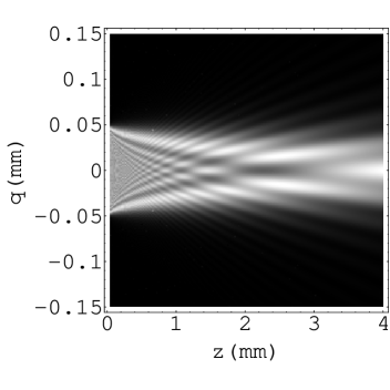
Fig. 1: Fresnel diffraction pattern for a one-dimensional aperture of width $0.1~{}\mathrm{mm}$ with $k=10^{7}$.

Fig. 1 shows a typical diffraction pattern obtained by numerical integration of Eq. (30).

For wide angles paraxial approximation no longer applies and the appropriate WDF transformation is now given by

$$W(\mathbf{q},\mathbf{p},z)=W(\mathbf{q}-\frac{z\mathbf{p}}{\sqrt{n^{2}-|\mathbf{p}|^{2}}},\mathbf{p},0)~{}~{} \rightarrow ~{}~{}|\mathbf{p}|<n,$$

$$W(\mathbf{q},\mathbf{p},z)=0~{}~{} \rightarrow ~{}~{}\mathrm{otherwise}.$$ (31)

Eq. (3) shows that only the moments such that $|\mathbf{p}|<n$ can be propagated [8]. In fact, if $|\mathbf{p}|/n=\sin\alpha$, with $\alpha$ the angle the ray makes with the $z$ axis, It is obvious that the higher moments would correspond to values of $|\sin\alpha|>1$; these moments don’t propagate and originate evanescent waves instead, Fig. 2. The net effect on near-field diffraction is that the high-frequency detail near the aperture is quickly reduced.

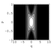
a)

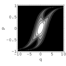
b)

Fig. 2: Propagation of the WDF in wide angle condition ($k=10^{6}~{}\mathrm{m}^{-1}$, horizontal scale in $\mu\mathrm{m}$). a) Original distribution, b) after propagation over $3~{}\mu\mathrm{m}$.

The field intensity can now be evaluated by the expression

$$\frac{k^{2}|\varphi(x,z)|^{2}}{4\pi^{2}} = \int_{p_{1}}^{p_{0}}{\frac{1}{kp_{x}}\sin\left\{kp_{x}\left[l-2\left(x-zp_{x}/\sqrt{n^{2}-p_{x}^{2}}\right)\right]\right\}dp_{x}}$$ (32)

$$+\int_{p_{0}}^{p_{2}}{\frac{1}{kp_{x}}\sin\left\{kp_{x}\left[l+2\left(x-zp_{x}/\sqrt{n^{2}-p_{x}^{2}}\right)\right]\right\}dp_{x}},$$

with

$$p_{0} = \frac{nx}{\sqrt{x^{2}+z^{2}}},$$

$$p_{1} = \frac{n(2x-l)}{\sqrt{(2x-l)^{2}+4z^{2}}},$$

$$p_{2} = \frac{n(2x+l)}{\sqrt{(2x+l)^{2}+4z^{2}}}.$$ (33)

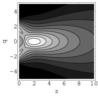
Fig. 3: Near-field diffraction pattern when the aperture width is exactly one wavelength; ($k=10^{6}~{}\mathrm{m}^{-1}$, both scales in $\mathrm{\mu m}$).

Fig. 3 shows the near-field diffraction pattern when the aperture is exactly one wavelength wide. The situation is such that all the high frequencies appear at values of $|p_{x}|>1$ and are evanescent, resulting in a field pattern with one small minimum immediately after the aperture, after which the beam takes a quasi-gaussian shape, without further minima. The width of the sharp peak just after the aperture is considerably smaller than one wavelength determining a super-resolution on this region.

4 Special relativity

Special relativity deals with a 4-dimensional space-time endowed with a pseudo-Euclidean metric which can be written as

$$ds^{2}=dx^{2}+dy^{2}+dz^{2}-dt^{2},$$ (34)

where the space-time is referred to the coordinates $(t,x,y,z)$. Here the units were chosen so as to make $c=1$, $c$ being the speed of light.

For a more adequate optical interpretation one can use coordinates $(x,y,z,\tau)$ with $\tau$ the proper time [9]:

$$\tau=t\left(1-\frac{v^{2}}{c^{2}}\right)^{1/2}=\frac{t}{\gamma}~{}.$$ (35)

Here $v^{2}=|\mathbf{v}|^{2}$, with $\mathbf{v}$

$$\mathbf{v}=\left(\frac{dx}{dt},\frac{dy}{dt},\frac{dz}{dt}\right),$$ (36)

the usual 3-velocity vector. Fig. 4 shows the coordinates of an event $\mathcal{E}$ when just two spatial coordinates are used together with coordinate $\tau$.

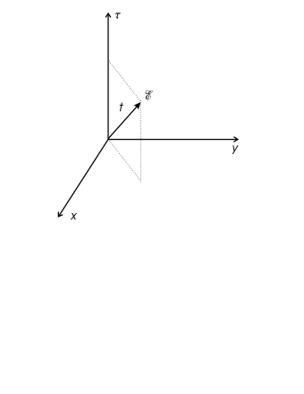
Fig. 4: The relativistic frame in two dimensions. The $\tau$ coordinate is the proper time while the distance to the origin is the time measured in the frame at rest.

Considering Eqs. (35, 36) and the new coordinates the metric defined by Eq. (34) becomes

$$ds^{2}=v^{2}dt^{2}-dt^{2}=d\tau^{2}.$$ (37)

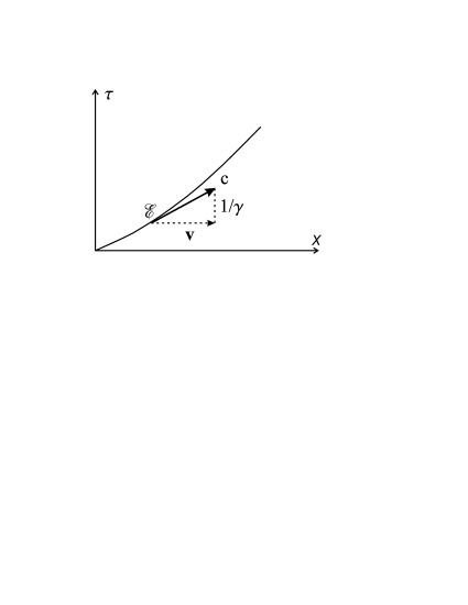
Fig. 5: The curved line represents the word line of event $\mathcal{E}$. The speed is represented by the vector $\mathbf{v}$, which is the side of a rectangular triangle whose hypotenuse has a magnitude $c$.

The trajectory of an event in 4-space is known as its world line. In Fig. 5 we represent the world line of an event $\mathcal{E}$ with coordinates $(x,\tau)$. At each position the derivative of the world line with respect to $\tau$ is

$$\dot{x}=\frac{dx}{dt}~{}\frac{dt}{d\tau}=\gamma v_{x}.$$ (38)

More generally we can write

$$\overrightarrow{\nu}=\gamma\mathbf{v},$$ (39)

with

$$\overrightarrow{\nu}=\left(\dot{x},\dot{y},\dot{z}\right).$$ (40)

It follows from Eq. (40) that, at each point, the components of $\mathbf{v}$ are the direction cosines of the tangent vector to the world line through that point.

We must now state a basic principle equivalent to Fermat’s principle for ray propagation in optics given in Eq. (1). Taking into consideration the relativistic Lagrangian we can state the following variational principle [3, 4]:

$$\delta\int{\left(m\gamma-V\right)ds}=0,$$ (41)

where $m$ is the rest mass of the particle and $V$ is the local potential energy. It can be shown that $m\gamma$ represents the kinetic energy of the particle. Using Eq. (37) a straightforward calculation shows that $ds=d\tau$ so that we can also write

$$\delta\int{\left(m\gamma-V\right)d\tau}=0.$$ (42)

The new principle means that the particle will choose a trajectory moving away from high potential energies much as the optical ray moves away from low refractive index. From this principle we can derive all the equations of relativistic mechanics, in a similar manner as from Fermat’s principle it is possible to derive light propagation.

Comparing this equation with Eq. (9), we can define the Lagrangian of the mechanical system as

$$L=\left(m\gamma-V\right).$$ (43)

We now have a 4-dimensional space, while in the Hamiltonian formulation of optics we used 3 dimensions. The following list shows the relationship between the two systems, where we refer first to the relativistic system and then to the optical system.

$$x \leftrightarrow x,$$

$$y \leftrightarrow y,$$

$$z \leftrightarrow \mathrm{no~{}equivalent},$$

$$\tau \leftrightarrow z.\$$

In the mapping from optical propagation to special relativity the optical axis becomes the proper time axis and the ray direction cosines correspond to the components of the speed vector $\mathbf{v}$. The refractive index has no direct homologous; it will be shown that in special relativity we must consider a non-homogeneous medium with different refractive indices in the spatial and proper time directions. We can derive the conjugate momentum from the Lagrangian using the standard procedure:

$$\mathbf{p}=\left(\frac{m\overrightarrow{\nu}}{\gamma}\right)=m\mathbf{v}.$$ (44)

Comparing with Eq. (2) it is clear that $m$ is the analogous of the position dependent refractive index.

The system Hamiltonian can be calculated

$$H = \mathbf{p}\cdot\mathbf{v}-L$$ (45)

$$= \frac{m\nu^{2}}{\gamma}-L$$

$$= -\frac{m}{\gamma}+V.$$

The canonical equations follow directly from Eq. (2)

$$\overrightarrow{\nu} = \gamma\mathbf{v},$$

$$\frac{d\mathbf{p}}{d\tau} = -\mathrm{grad}H,$$ (46)

where the gradient is taken over the spatial coordinates, as usual.

The first of the equations above is the same as Eq. (40), while the second one can be developed as

$$\frac{d}{d\tau}\left(\frac{m}{\gamma}\overrightarrow{\nu}\right)=\mathrm{grad}\left(\frac{m}{\gamma}-V\right).$$ (47)

Considering that from the quantities inside the gradient only the potential energy should be a function of the spatial coordinates, we can simplify the second member:

$$\frac{d}{d\tau}\left(\frac{m}{\gamma}\overrightarrow{\nu}\right) = -\mathrm{grad}V$$ (48)

$$\frac{d}{d\tau}\left(m\mathbf{v}\right) = -\mathrm{grad}V.$$ (49)

Eq. (49) is formally equivalent to the last two Eqs. (2), confirming that the conjugate momentum components are proportional to world line’s direction cosines in 4-space. The total refractive index analogue can now be found to be $m-V/\gamma$. We can check the validity of Eq. (49) by replacing the $\tau$ derivative by a derivative with respect to $t$.

$$\frac{d}{dt}\left(m\gamma\mathbf{v}\right)=-\mathrm{grad}V,$$ (50)

where $m\gamma$ is the relativistic mass and the product $m\gamma\mathbf{v}$ is the relativistic momentum.

If the mass is allowed to be coordinate dependent, as a mass distribution through the Universe, the passage between Eqs. (47) and (48) is illegitimate and we are led to equations similar to Eq. (2). The consideration of a coordinate dependent mass allows the prediction of worm tubes, the analogues of optical waveguides, and black holes, which would have optical analogues in high refractive index glass beads with gradual transition to vacuum refractive index.

5 De Broglie’s wavelength

The formal equivalence between light propagation and special relativity in the $x,y,z,\tau$ frame suggests that de Broglie’s wavelength may be the formal equivalent of light wavelength. We would like to associate an event’s world line to a light ray and similarly we want to say that, in the absence of a potential, the event’s world line is the normal to the wavefront at every point in 4-space. We must start from a basic principle, stating that each particle has an intrinsic frequency related to it’s mass in a similar way as the wavelength of light is related to the refractive index; we state this principle by the equation

$$f=\frac{m}{h},$$ (51)

where $h$ is Planck’s constant. If we remember that everything is normalized to the speed of light by $c=1$, Eq. (51) is equivalent to a photon’s energy equation

$$E=hf.$$ (52)

So we have extended an existing principle to state that any particle has an intrinsic frequency that is the result of dividing it’s equivalent energy $E=mc^{2}$ by Planck’s constant.

In the 4-space $x,y,z,\tau$ frame a material particle travels in a trajectory with direction cosines given by the components of $\mathbf{v}$ and consistently a photon travels along a spatial direction with zero component in the $\tau$ direction. The intrinsic frequency defined by Eq. (51) originates a wavelength along the world line given by

$$\lambda_{w}=\frac{c}{f}=\frac{h}{mc},$$ (53)

where we have temporarily removed the $c$ normalization for clarity reasons.

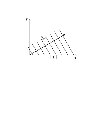
Fig. 6: The moving particle has a world wavelength $\lambda_{w}=h/(mc)$ and a spatial wavelength $\lambda=h/(mv)$.

As shown in Fig. 6, when projected onto 3-space $\lambda_{w}$ defines a spatial wavelength such that

$$\lambda=\frac{\lambda_{w}c}{v}=\frac{h}{p}.$$ (54)

The previous equation defines a spatial wavelength which is the same as was originally proposed by de Broglie in the non-relativistic limit. When the speed of light is approached Eq. (54) will produce a wavelength $\lambda\rightarrow\lambda_{w}$ while de Broglie’s predictions use the relativistic momentum and so $\lambda\rightarrow\infty$ when $v\rightarrow c$.

6 Wave propagation and Schrödinger equation

The arguments in the previous paragraphs lead us to state the general principle that a particle has an associated frequency given by Eq. (51) and travels on a world line through 4-space with the speed of light. In a generalization to wave packets, we will respect the formal similarity with light propagation and state that all waves travel in 4-space with the speed of light. A particle about which we know mass and speed but know nothing about its position will be represented by a monocromatic wave and a moving particle in general will be represented by a wave packet.

According to general optical practice we will say that the field must verify the wave equation

$$\left(\nabla^{2}-\frac{\partial^{2}}{\partial t^{2}}\right)\varphi(\mathcal{P},t)=0,$$ (55)

where $\mathcal{P}$ is a point in 4-space and $\nabla^{2}$ is an extended laplacian operator

$$\nabla^{2}=\frac{\partial^{2}}{\partial x^{2}}+\frac{\partial^{2}}{\partial y^{2}}+\frac{\partial^{2}}{\partial z^{2}}+\frac{\partial^{2}}{\partial\tau^{2}}.$$ (56)

In Eq. (55) we have returned to the $c=1$ normalization in order to treat all the coordinates on an equal footing. Due to the special 4-space metric we will assume that $\varphi(\mathcal{P},t)$ is of the form

$$\varphi(\mathcal{P},t)=\Phi(\mathcal{P})e^{i2\pi ft},$$ (57)

with $f$ given by Eq. (51). Notice that we used a plus sign in the exponent instead of the minus sign used in optical propagation; this is due to the special 4-space metric.

Not surprisingly we will find that, in the absence of a potential, Eq. (55) can be written in the form of Helmoltz equation

$$\left(\nabla^{2}+k^{2}\right)\Phi(\mathcal{P})=0,$$ (58)

with

$$k=\frac{2\pi}{\lambda_{w}}.$$ (59)

If we take into consideration Eq. (35), the laplacian becomes

$$\nabla^{2} = \frac{\partial^{2}}{\partial x^{2}}+\frac{\partial^{2}}{\partial y^{2}}+\frac{\partial^{2}}{\partial z^{2}}+\gamma^{2}\frac{\partial^{2}}{\partial t^{2}}$$ (60)

$$= \nabla_{3}^{2}+\gamma^{2}\frac{\partial^{2}}{\partial t^{2}},$$

where $\nabla_{3}^{2}$ represents the usual laplacian operator in 3-space.

In order to derive Schrödinger equation we re-write Eq. (55)

$$\nabla^{2}\varphi(\mathcal{P},t)+ik\frac{\partial\varphi(\mathcal{P},t)}{\partial t}=0,$$ (61)

and using Eq. (60)

$$\nabla_{3}^{2}\varphi(\mathcal{P},t)+ik(\gamma^{2}+1)~{}\frac{\partial\varphi(\mathcal{P},t)}{\partial t}=0.$$ (62)

In a non-relativistic situation $\gamma\rightarrow 1$. Considering Eq. (53) we can write Eq. (62) in the form of Schrödinger equation [10]

$$i\hbar\frac{\partial\varphi(\mathcal{P},t)}{\partial t}=-\frac{\hbar^{2}}{2m}\nabla_{3}^{2}\varphi(\mathcal{P},t),$$ (63)

where $\hbar=h/(2\pi)$.

Eq. (63) retains the symbol $\mathcal{P}$ representing a point in 4-space. It must be noted, though, that in a non-relativistic situation $\tau\rightarrow t$ and we can say that $\varphi(\mathcal{P},t)\rightarrow\varphi(P,t)$ with $P$ having the 3-space coordinates of $\mathcal{P}$.

In the presence of a potential we have to consider that momentum is no longer preserved, as shown by Eq. (49). This can be taken into account when we evaluate the laplacian in Eq. (62) by the inclusion of an extra term $-V\varphi(\mathcal{P},t)$. We will the end up with the Schrödinger equation in a potential.

7 Heisenberg’s uncertainty principle

For the pair of associated variables $x$ and $p_{x}$, Heisenberg’s uncertainty principle states that there is an uncertainty governed by the relation

$$\Delta x\Delta p_{x}\geq\frac{\hbar}{2}.$$ (64)

The interpretation of the uncertainty principle is that the best we know a particle’s position, the least we know about its momentum and vice-versa; the product of the position and momentum distribution widths is a small number multiplied by Planck’s constant. An application of the uncertainty relationship is usually found in the diffraction of a particle by an aperture.

If we assume that the localization of a particle with momentum $p_{x}$ can be done with an aperture of width $\Delta x$, we can use Fraunhofer diffraction theory to say that further along the way the probability of finding the particle with any particular value of it’s momentum will be given by the square of the aperture Fourier transform, considering de Broglie’s relationship for the translation of momentum into wavelength.

A rectangular aperture of width $\Delta x$ has a Fourier transform given by

$$A(f_{x})=\Delta x\mathrm{~{}sinc}(\Delta xf_{x}),$$ (65)

where $\mathrm{sinc}$ is the usual $\sin(x)/x$ function.

Considering de Broglie’s relationship given by Eq. (54), making $f_{x}=1/\lambda$ and the fact that the Fourier transform must be squared we can write

$$P(p_{x})=\Delta x^{2}\mathrm{~{}sinc}^{2}\left(\frac{\Delta xp_{x}}{h}\right).$$ (66)

The second member on the previous equation has its first minimum for $\Delta xp_{x}/h=\pi$ and so we can say that the spread in momentum is governed by $\Delta x\Delta p_{x}=\pi h$ and Eq. (64) is verified.

If we accept that wave packets propagate in 4-space at the speed of light and that the momentum is given by Eq. (44), there is a upper limit to the modulus of the momentum $|\mathbf{p}|\leq mc$. In the propagation of light rays we found a similar limitation as $|\mathbf{p}|\leq n$ with the results in light diffraction exemplified by Eq. (32) and Fig. 3. It is expected that the same effects will be present in particle diffraction and in fact Figs. 2 and 3 could also represent the diffraction of a stationary particle by an aperture with width equal to $\lambda_{w}$. The strong peak about half one wavelength in front of the aperture shows that the particle is localized in a region considerably smaller than its wavelength and, above all, shows the inexistence of higher order peaks.

8 Conclusions

Special relativity was shown to be formally equivalent to light propagation, provided the time axis is replaced by the proper time. In this coordinate set all particles follow w world line at the speed of light and can be assumed to have an intrinsic frequency given by $mc^{2}/h$. Quantum mechanics is then a projection of 4-space wave propagation into 3-space. Important conclusions were possible through the analogy with light propagation and diffraction.

It was possible to derive Schrödinger equation and it was shown that Heisenberg’s uncertainty principle may be violated in special cases in the very close range, similarly to what had already been shown to happen in light diffraction [1].

Future work will probably allow the derivation of relativistic quantum mechanics conclusions, through the use of the Wigner Distribution Function for the prediction of wave packet propagation in 4-space.

9 Acknowledgements

The author acknowledges the many fruitful discussions with Estelita Vaz from the Mathematics Department of Universidade do Minho, especially on the subject of relativity.

References

- [1] J. B. Almeida and V. Lakshminarayanan, ”Wide Angle Near-Field Diffraction and Wigner Distribution”, Submitted to Opt. Lett. (unpublished).
- [2] M. Born and E. Wolf, Principles of Optics, 6th. ed. (Cambridge University Press, Cambridge, U.K., 1997).
- [3] H. Goldstein, Classical Mechanics, 2nd. ed. (Addison Wesley, Reading, MA, 1980).
- [4] V. J. José and E. J. Saletan, Classical Mechanics – A Contemporary Aproach, 1st. ed. (Cambridge University Press, Cambridge, U.K., 1998).
- [5] M. J. Bastiaans, “The Wigner Distribution Function and Hamilton’s Characteristics of a Geometric-Optical System,” Opt. Commun. 30, 321–326 (1979).
- [6] D. Dragoman, “The Wigner Distribution Function in Optics and Optoelectronics,” in Progress in Optics, E. Wolf, ed., (Elsevier, Amsterdam, 1997), Vol. 37, Chap. 1, pp. 1–56.
- [7] M. J. Bastiaans, “Application of the Wigner Distribution Function in Optics,” In The Wigner Distribution - Theory and Applications in Signal Processing, W. Mecklenbräuker and F. Hlawatsch, eds., pp. 375–426 (Elsevier Science, Amsterdam, Netherlands, 1997).
- [8] J. W. Goodman, Introduction to Fourier Optics (McGraw-Hill, New York, 1968).
- [9] R. D’Inverno, Introducing Einstein’s Relativity (Clarendon Press, Oxford, 1996).
- [10] S. Gasiorowicz, Quantum Physics, 2nd ed. (J. Wiley and Sons, New York, 1996).