On Optimality in Auditory Information Processing

Abstract

We study limits for the detection and estimation of weak sinusoidal signals in the primary part of the mammalian auditory system using a stochastic Fitzhugh-Nagumo (FHN) model and an action-reaction model for synaptic plasticity. Our overall model covers the chain from a hair cell to a point just after the synaptic connection with a cell in the cochlear nucleus. The information processing performance of the system is evaluated using so called $\phi$-divergences from statistics which quantify a dissimilarity between probability measures and are intimately related to a number of fundamental limits in statistics and information theory (IT). We show that there exists a set of parameters that can optimize several important $\phi$-divergences simultaneously and that this set corresponds to a constant quiescent firing rate (QFR) of the spiral ganglion neuron. The optimal value of the QFR is frequency dependent but is essentially independent of the amplitude of the signal (for small amplitudes). Consequently, optimal processing according to several standard IT criteria can be accomplished for this model if and only if the parameters are “tuned” to values that correspond to one and the same QFR. This offers a new explanation for the QFR and can provide new insight into the role played by several other parameters of the peripheral auditory system.

1 Introduction

When a sensory cell in a mammal is presented with a stimulus, the information about it must in general be communicated through several layers of intermediating nerve cells before it reaches the parts of the brain where the final processing takes place. A logical question, therefore, is how much of the information is lost in the first parts of this processing chain and how have these parts of the chain have (possibly) been optimized by evolution to combat information loss, for different types of stimuli. One of the simplest settings of this problem is the auditory system. The frequency filtering process in the inner ear makes it sufficient in general, at least for weak signals, to restrict attention to a single type of stimuli, a pure tone, when studying the response of the auditory nerve cells and their connections in the cochlear nucleus. From an information-theoretic perspective it is thus of interest to determine how well the peripheral parts of the auditory processing chain preserve information about the two parameters, the amplitude and phase, that characterize a tone at a given frequency. An even more fundamental question, however, is how well information about the presence of such a tone is preserved, i.e. in what ways this part of the auditory processing chain imposes limits on achievable detection performance. Mathematically, these two problems belong to the realm of statistical decision and information theory (IT); for weak tones the detection problem is, moreover, intimately connected with the estimation problem of determining the amplitude.

Despite the extensive literature on information processing in neurons, a relatively small number of works treat the fundamental statistical limits for neural detection and estimation that bound the performance of sensory systems. One notable exception, however, is Stemmler’s work [Stemmler (1996)] on the detection and estimation capabilities of the Hodgkin-Huxley, McCullough-Pitts and leaky integrate-and-fire model neurons in terms of the Fisher Information. Stemmler shows that there exists a universal small-signal scaling law which relates the optimal detection, estimation, and communication performance of these model neurons, and that this scaling law also applies to the (narrow-band) signal-to-noise ratio (SNR) on the output of a neuron which is excited by a sinusoidal signal. Manwani and Koch [Manwani and Koch (1999)] give a detailed analysis of the noise in dendritic cable structures and its effect on fundamental limits for detection and estimation. In particular, they provide relations for minimum mean-square error in linear estimation and minimum probability of error (the latter under an assumption of Gaussian noise) based on a stochastic version of the linear one-dimensional cable equation. In the majority of other information theoretic analyses of neural information processing the focus is on the spike train on the output of a neuron though, and a long-standing objective has been to try to break the “neural code” of the spike train. However, there is a fundamental component missing in modeling that rests solely on considering information in the spike train and it is the influence of the synaptic connections. The importance of this aspect of neural computation has recently been recognized and it has even been suggested that the synaptic connections in fact represent the primary bottleneck that limits information transmission in neural circuitry [Zador (1998)]. Consequently, when studying information processing in neurons, in particular detection and estimation capabilities of the auditory system, it seems imperative to consider models and methods that describe not only the individual neurons and their spike trains but also the synaptic connections between the neurons.

In the present study we investigate, theoretically, the fundamental limits for detection and estimation of weak signals in the mammalian auditory system. We model the neurons in the auditory nerve and their synaptic connections using ideas from Tuckwell [Tuckwell (1988)] and Kistler-Van Hemmen [Kistler and Van Hemmen (1999)] that take into account the notion of synaptic plasticity. Incorporation of the synaptic efficacy’s dependence on the prehistory of action potentials arriving to the synapse in the model makes it possible to obtain a more realistic assessment of the information available to the next step in the auditory processing chain, the processing in the cochlear nucleus. Another feature of our study is the use of more general measures of signal-noise separation. To quantify signal-noise separation we use the so-called $\phi$-divergences from statistics and IT [Liese and Vajda (1987)]. The $\phi$-divergences are applicable to virtually any kind of signal and system (in a stochastic setting), in particular the highly nonlinear dynamic systems represented by neurons, and are intimately related to a number of fundamental limits in statistics/IT. Our main objective is to determine whether the primary auditory system has a structure whereby (nontrivial) optimizations of $\phi$-divergences with respect to parameters can occur. Given the significance of the $\phi$-divergences as performance measures, an affirmative answer to this question would yield a new view on the role played by various parameters in the neurons of the auditory system, such as the quiescent firing rate (QFR), and would inspire new experiments relating to the function of the auditory processing chain. We show that such optimizations indeed are possible, where some of the underlying mechanisms are explained in terms of the model structure, and we numerically determine the optimal values.

The paper is organized as follows. In Section 2 we describe our model of the auditory system, in which the central component are the Fitzhugh-Nagumo equations. This section also includes an introduction to $\phi$-divergences and a review of their properties. The divergences are computed in Section 3, and discussed in Section 4.

2 Methods

2.1 Physiological modeling

We consider the peripheral part of the mammalian auditory nervous system [Geisler (1998)], beginning with the acoustic (fluid) pressure at a point in the inner ear and ending at the soma of a cell in the cochlear nucleus. As a model of the chain from the inner ear, via an inner hair cell and a spiral ganglion cell, to a point a small distance down the ganglion axon we employ a stochastic FitzHugh-Nagumo (FHN) model [FitzHugh (1961), Scott (1975)]. This model, which we henceforth (with a slight abuse of language) will call the FHN neuron, represents an attractive choice in our study for two reasons: It is analytically/numerically tractable and has the ability to produce a response that is both visually and statistically similar to that observed in real neurons. In particular, it is well-known that even simple (white-noise driven) stochastic FHN models are able to accurately reproduce the interspike interval histograms (ISIH) in various forms of nerve fibers, such as the auditory nerve fibers of squirrel monkeys [Massanes and Vicente (1999)]. For the terminal boutonic connections of the auditory nerve with the dendrites (or soma) of the cells in the cochlear nucleus, together with the parts of the dendrites from the boutonic connections to the somas, we employ an action-reaction model combined with a time-varying $\alpha$-function like transformation with additive noise [Tuckwell (1988), Kistler and Van Hemmen (1999)]. The conjunction of these two model features makes it possible to capture both the synaptic plasticity and variability observed in real neurons. Furthermore, incorporation of plasticity in the model turns out to be of crucial importance for our results since it removes “false optima” that would otherwise be present.

2.1.1 Stochastic FitzHugh-Nagumo Model.

The stochastic FHN model is given by the following system of stochastic differential equations [Longtin (1993)]

$$\begin{array}[]{rcl}\varepsilon dV_{t}&=&V_{t}(V_{t}-a)(1-V_{t})\,dt-W_{t}\,dt+dv_{t},\\ dW_{t}&=&(V_{t}-\delta W_{t}-(b+s_{t}))\,dt,\\ \end{array},\quad t\in[0,T],$$ (1)

where $\varepsilon,a,b,\delta>0$ are (nonrandom) parameters, $V$ is the fast (“voltage like”) variable, $W$ is the slow (“recovery like”) variable, and $s_{t}$ is the signal process representing the stimuli, here the acoustic pressure in the inner ear. The parameter $a$ effectively controls the barrier height between the two potential wells in the potential term (i.e., the first term on the RHS of the first equation) and the variable $b$ is a bias parameter moderating the effect of the signal input. These two parameters affect the stability properties of the FHN neuron, and so does the relaxation parameter $\delta$ multiplying the slow variable. The parameter $\varepsilon$ sets the time scale for the motion in the potential described by the first equation. Normally, the variable $V$ is thought to represent membrane voltage in the neuron but since the FHN model can be viewed as obtained by “descent” from the higher dimensional Hodgkin-Huxley model (or other likewise more elaborated models) it is not reasonable to attach a too strict physical meaning to it. To us it will merely act as a convenient way of modeling the timing information in the action potentials generated by the neuron when the latter are defined via a simple threshold operation on the fast variable $V$. The signal $s_{t}$ is here chosen to enter on the slow variable $W$, which controls the refractory periods of $V$, in order to facilitate a comparison with the qualitative results for the corresponding deterministic dynamics in [Alexander et al. (1990)]. However, it is easy to transform the system into an equivalent one (of the same form) where the signal enters on the fast variable [Alexander et al. (1990)]. The stochastic process $v_{t}$ is a noise process accounting for the variability in firing pattern observed in real neurons, which we in order to have control over the correlation time [Longtin (1993)] take to be an Ornstein-Uhlenbeck (OU) process

$$dv_{t}=-\lambda v_{t}\,dt+\sigma d\xi_{t},\quad t\in[0,T],$$ (2)

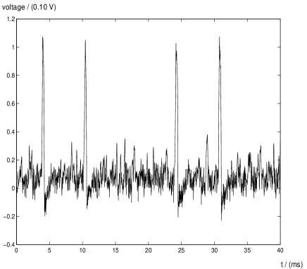
Figure 1: A typical example of the output from the model (1),(2) with parameters $a=0.55$, $b=0.12$, $\delta=1$, $\varepsilon=0.005$, $\sigma=100\sqrt{2\cdot 10^{-5}}$ and $\lambda=100$, when an input signal $s_{t}$ as in (5) with parameters $A=0.1$ and $\omega_{0}=8$ is applied.

where $\lambda>0$ determines the effective correlation time and $\sigma>0$ is the intensity of a standard Wiener process (integrated Gaussian white noise) $\xi$. We assume that all the input and intrinsic noise sources can be collectively described by this process. This noise model is also often used with $\lambda=0$, so that $v_{t}$ becomes a Wiener process, which has proved sufficient to reproduce real data, see e.g. [Massanes and Vicente (1999)]. An example of an output to the FHN neuron (1),(2) with sinusoidal signal and parameter values typical for the simulations is shown in Fig. 1.

2.1.2 Spike train.

An important underlying assumption in our model and, indeed, in most rate-based treatments of neural dynamics, is that the intervals between action potentials, not their particular form, in a given neuron carry all the information relevant to the subsequent neural processing by other connected neurons. Accordingly, in the remaining parts of the model that describe how the output of the FHN neuron is processed we replace the output of the FHN neuron by an equivalent random point process

$$\mathcal{T}=\{0<\tau_{0}<\dots<\tau_{k-1}<\tau_{k}<\tau_{k+1}\dots\leq T\},$$

(the number of points in $\mathcal{T}$ may be finite or infinite) where $\tau_{k}$ is defined by level crossings of the fast variable $V$ in the FHN model as

$$\tau_{k+1}=\inf\{t>\tau_{k}:V_{t}>\gamma\mbox{ and }V_{s}<\gamma\mbox{ for some }\tau_{k}\leq s\leq t\}.$$

In other words, $\tau_{k+1}$ is the first time after $\tau_{k}$ for an upcrossing over the level $\gamma$ ($\tau_{0}$ is the first time for an upcrossing after $t=0$), where $\gamma$ is suitably chosen to represent an action potential level. The point process $\mathcal{T}$ thus contains the timing information in the nerve signals at a point in the auditory nerve immediately after the ganglion cell and will therefore be referred to as the spike train. Since the shapes and relative positions of the action potentials are not appreciably changed as they propagate through the (myelinated) axons of the auditory nerve we assume that the process $\mathcal{T}$ also represents the timing information in the action potentials as they reach a terminal connection in the telodendria of the ganglion cell.

2.1.3 Synaptic connections.

The model for synaptic response is made up of two parts; a nominal (or average) response and a variability from the nominal due to synaptic plasticity [Koch (1999), ch. 13].

For a synapse in a nominal state at an electrotonic distance $x_{0}$ from the soma on a dendrite of some length $L\geq x_{0}$, the impulse response $r$ (“Green’s function”) for the transformation from action potential applied on the presynaptic side of the synapse to the voltage at the soma can be modeled by an expansion of the form [Tuckwell (1988), sec. 6.5]

$$r(t)=\beta\sum_{n=0}^{\infty}\frac{A_{n}(x_{0})}{1+\lambda_{n}^{2}-\alpha}\Big{(}te^{-\alpha t}-\frac{e^{-\alpha t}+e^{-t(1+\lambda_{n}^{2})}}{1+\lambda_{n}^{2}-\alpha}\Big{)},\quad t\geq 0,$$ (3)

(with uniform convergence) where $r(t)=0$ for $t<0$. Expressions for the constants $A_{n},\lambda_{n}$ in terms of $L$, and graphs showing the appearance of (3) for typical values of these constants and $\alpha,\beta$, are given in [Tuckwell (1988)]. In (3) it is assumed that the impulse response from action potential to post-synaptic current at the soma is given by a so-called $\alpha$-function of the form $h(t)=\beta te^{-t\alpha}$ for $t\geq 0$ and $h(t)=0$ for $t<0$ [Jack and Redman (1971)]. From the definition of $r$ it is clear that the expression (3) actually describes both the synapse and a part of the dendrite (the part between the synapse and the soma), but since the response at a point down the dendrite is mainly determined by the response of the synapse we shall, for simplicity, refer to $r$ in (3) as the nominal synaptic response.

The synaptic connections in the cochlear nucleus are often made by synapses having a fair, or even a large amount, of release sites, such as the endbulb of Held, which is connected to spherical bushy cells in the anteroventral cochlear nucleus [Webster et al. (1992)]. As a consequence, the synaptic transmission will be reliable in the sense that an incoming action potential will almost always yield an excitatory postsynaptic potential (EPSP). However, the EPSPs will vary in strength depending (primarily) on the prehistory of the action potentials that have arrived at the synapse. This phenomenon, the synaptic plasticity, has a crucial effect on the overall dynamical behavior of the nerve and needs to be taken into account in conjunction with the nominal response in (3). We model the plasticity using a simple action-recovery scheme developed by Kistler and Van Hemmen [Kistler and Van Hemmen (1999)] which combines the three state plasticity model of Tsodyks and Markham [Tsodyks and Markham (1997)] and the spike response model of Gerstner and van Hemmen [Gerstner and Van Hemmen (1992)]. The action-recovery scheme employs a variable $Z$ and its complement $1-Z$ that correspond to “active” and “inactive” resources, respectively, where the term “resources” can be interpreted as resources on both the pre- and the postsynaptic side, such as the availability of neurotransmitter substance or postsynaptic receptors. In addition, resources can also be interpreted as some ionic concentration gradient, e.g. the membrane potential on the postsynaptic side. This approach, therefore, also compensates for the EPSPs’ dependence on the voltage of the following neuron’s soma. Quantitatively, the amount of available resources are determined by the recursion [Kistler and Van Hemmen (1999)]

$$Z_{\tau_{k}+1}=1-[1-(1-R)Z_{\tau_{k}}]\exp[-(\tau_{k+1}-\tau_{k})/\tau],$$ (4)

where $0<R\leq 1$ is a constant corresponding to the fraction of resources that gets inactive due to a spike and $\tau>0$ is a decay time parameter. The variable $Z_{\tau_{k}}$ should be interpreted as the amount of resources available just before time $\tau_{k}$ and it is therefore proportional to the strength in an eventual EPSP caused by an action potential arriving to the synapse at time $\tau_{k}$. An approximation to the initial condition $Z_{\tau_{0}}$ can be obtained by forming an average of the available resources for a number of spike trains, generated by the unforced FHN model for the studied system, for a large $T$. Thus, by using the plasticity model above we can calculate the pristine (or noise-free) postsynaptic response $R$ as

$$R(t,x)=\sum_{k=0}^{\infty}Z_{\tau_{k}}r(t-\tau_{k}),\quad t>0,$$

where $r$ is the nominal response given in (3). This model is capable of producing results in close agreement with real data (cf. [Tsodyks and Markham (1997)]), provided the appropriate choices of constants are made.

In reality there is always also a certain noise present due to e.g. the inherent unreliability of the ionic channels involved in the transmission of signals in and between the neurons [Koch (1999)]. To take this effect into account we have added zero mean white Gaussian noise with intensity $\sigma_{2}$ to the EPSPs given by our model, which thus represents our total synaptic response.

2.2 Information processing

We study information processing performance in terms of general statistical signal-noise separation measures applied to the output of our model, the soma of a cell in the cochlear nucleus. The output signal-noise separation setting was chosen since it can be applied with only minimal assumptions about the input signal. Due to the frequency selectivity of the primary parts of the auditory system it is sufficient, at least as a good first approximation for weak signals [Eguíluz et al. (2000), Camalet et al. (2000)], to restrict attention to sinusoidal signals (possibly with slowly varying amplitude and phase). The simplicity that the output-separation setting offers can be contrasted with that of a communications setting which in general would require considerably more assumptions in order to define quantities like alphabet, message, coding and channel capacity [Cover and Thomas (1991)]. Of course, one could also select some stochastic signal and consider only mutual information between input and output but this too would require some further statistical assumptions. For our study however, it is sufficient to restrict attention to the very simple class of signals $s_{t}$ in the FHN model of the form

$$s_{t}=A\sin(\omega_{0}t+\varphi),$$ (5)

where $A,\omega\geq 0$ are constant in time and $\varphi\in[-\pi,\pi)$ is a phase which is also constant in time.

2.2.1 $\phi$-divergences and generalized SNR.

A number of fundamental limits in statistical inference and IT can be expressed as monotonic functions of so-called $\phi$-divergences, which can be though of as “directed distances” between probability measures. For example, the minimal probability of error in (Bayesian) detection, Wald’s inequalities (sequential detection), the bound in Stein’s lemma (cutoff rates in Neyman-Pearson detection) and the Fisher information for small parameter deviations (the Cramér-Rao bound) can all be written as simple functions of a $\phi$-divergence. In the simplest setting, where $p_{0},p_{1}$ are two probability density functions (PDFs) on the real line $\mathbb{R}$, the $\phi$-divergence $d_{\phi}(p_{0},p_{1})$ between $p_{0},p_{1}$ is defined as [Liese and Vajda (1987)]

$$d_{\phi}(p_{0},p_{1})=\int_{\mathbb{R}}\phi\Big{(}\frac{p_{1}(x)}{p_{0}(x)}\Big{)}p_{0}(x)\,dx,$$ (6)

where $\phi$ is any continuous convex function $\phi$ on $[0,\infty)$ (we assume $p_{0}(x)=0$ if $p_{1}(x)=0$). A $\phi$-divergence satisfies $d_{\phi}(p_{0},p_{1})\geq 0$, with equality if and only if $p_{0}=p_{1}$ almost everywhere, and thus expresses the “separation” between $p_{0},p_{1}$ in a relative-entropy like way. Indeed, one prominent member of the family of $\phi$-divergences is the Kullback-Liebler divergence or relative entropy, also known as information divergence $d_{I}$ [Cover and Thomas (1991)], obtained for $\phi(x)=-\ln(x)$. Other important members of this family are the Kolmogorov or error divergence $d_{\mathcal{E}}^{(q)}$, obtained for $\phi(x)=|(1-q)x-q|$ where $q\in[0,1]$ is a parameter, and the $\chi^{2}$-divergence $d_{\chi^{2}}$, obtained for $\phi(x)=(1-x)^{2}$.

The $\chi^{2}$-divergence is twice the first term in a formal expansion of the information divergence around 0 (i.e. for $p_{0}=p_{1}$) and is a (tight) upper bound for a family of generalized SNR measures known as deflection ratios that depend only on the means and variances of the observables. If $h$ is some function of data, the deflection ratio (DR) $D(h)$ is defined as [Basseville (1989)]

$$D(h)=\frac{|E_{1}(h)-E_{0}(h)|^{2}}{\mbox{Var}_{0}(h)},$$

where $E_{1}(h),E_{0}(h)$ is the expectation of $h$ computed using $p_{0}$ and $p_{1}$, respectively, and $\mbox{Var}_{0}(h)$ is the variance of $h$ computed using $p_{0}$. The DR is upper-bounded as

$$D(h)\leq d_{\chi^{2}}(p_{0},p_{1}),$$ (7)

with equality if and only if $C_{1}(h-E_{0}(h))=C_{2}(p_{1}/p_{0}-1)$ with $p_{0}$-probability one, for two constants $C_{1},C_{2}$ not both zero. In particular, we have equality in (7) if $h$ equals $p_{1}/p_{0}$, the likelihood ratio. It follows that a larger $\chi^{2}$-divergence allows for larger SNR, when expressed in terms of DRs.

The $\chi^{2}$ and information divergences determine locally the Cramér-Rao bound (CRB) for parameter estimation ([Salicru (1993), Cover and Thomas (1991)]). For example, if $\theta$ is a parameter with values in some open interval $\mathcal{I}$ and $p_{\theta},\theta\in\mathcal{I},$ is a family of PDFs on $\mathbb{R}$ indexed by $\theta$ then, under some regularity conditions,

$$\lim_{\theta\rightarrow\theta_{0}}\frac{d_{I}(p_{\theta_{0}},p_{\theta})}{(\theta-\theta_{0})^{2}}=\lim_{\theta\rightarrow\theta_{0}}\frac{d_{\chi^{2}}(p_{\theta_{0}},p_{\theta})}{2(\theta-\theta_{0})^{2}}=\frac{1}{2}I(\theta_{0}),$$

for $\theta_{0}\in\mathcal{I}$, where $I(\theta_{0})$ is the Fisher Information at $\theta_{0}$. Thus, for estimation of $\theta$ when $\theta$ is near $\theta_{0}$ the CRB (which is the inverse of the Fisher Information), and thereby the achievable accuracy for unbiased estimation of $\theta$, is locally determined by the growth of the $\chi^{2}$ and information divergences as a functions of $\theta$, near $\theta_{0}$.

The Kolmogorov divergence is directly related to the minimal achievable probability of error in Bayesian hypothesis testing. If $p_{0}$ and $p_{1}$ are two possible PDFs for the data observed and $q$ is taken as the a priori probability of $p_{0}$ to be correct, so that $p_{1}$ has probability $1-q$, then the minimal achievable probability of error $\tilde{P}_{e}^{(q)}(p_{0},p_{1})$ for decision between $p_{0},p_{1}$ (i.e. which is the correct density) based on a single sample $x$ is given by (cf. e.g. [Ali and Silvey (1966)])

$$\tilde{P}_{e}^{(q)}(p_{0},p_{1})=\frac{1}{2}\big{(}1-d_{\mathcal{E}}^{(q)}(p_{0},p_{1})\big{)}.$$

A larger Kolmogorov divergence thus gives a smaller minimal probability of error.

For later reference we point out that all the definitions and properties above have counterparts on much more general probability spaces [Liese and Vajda (1987), Robinson et al. (2000), Rung and Robinson (2000)], for instance in the infinite dimensional context of probability measures on the space of continuous functions on $[0,T]$.

2.2.2 Auditory processing performance.

In order to apply $\phi$-divergences to assess performance in our model of the auditory processing chain, we need to specify the setting in somewhat greater detail, as well as elaborate some of the features of the model.

We have chosen to make the parameters $A,\omega$ and $\varphi$ constant, which in a detection scenario means that we are considering so-called coherent detection (detection of a completely deterministic signal). At first this might seem as an oversimplification but we argue that it is not, for the following reason. There are a number of nerve cells in the auditory nerve “tuned” to any given frequency and each corresponding axon, moreover, exhibits spatial divergence near the end where it splits up into different branches. Connections are then made between these branches and the dendritic tree or soma of the following neurons. Since the dendrites (from the connective synapse to the soma) have different lengths, the time delays in them will be different. For sinusoidal input signals this can be exchanged for a phase shift of the signal, at least as a good first approximation. Thus, for a given frequency, the primary auditory processing can be viewed as taking place over a “bank” of parallel channels, similar in characteristics but corresponding to different phase shifts. In a detection setting this corresponds to a bank of coherent detectors operating on the outputs of these channels. It is conceivable that the subsequent processing can take advantage of this low-level parallelism and that detection is possible based on a logical “or” operation where one detector indicating presence of the signal is sufficient. Therefore, we use a fixed phase $\varphi$ in the signal $s_{t}$ in (1),(5) and treat the phase as a (variable) parameter.

We assess the auditory processing performance by computing the $\phi$-divergences of the output of our model (the voltage to the soma of a cell in the cochlear nucleus) at a time point $T$, where $T$ is the end point of a long time interval $[0,T]$. The two PDFs $p_{0},p_{1}$ in the definition (6) are in the present setting given by the PDF for the output when no signal is present in the FHN model (1),(2) (i.e. $s_{t}\equiv 0$) and when a signal $s_{t}$ as in (5) is present, respectively. Since the PDFs in this case are densities on the real line they are easy to compute, using numerical simulation, but they are dependent on the phase $\varphi$, and so are the resulting $\phi$-divergences. In order to overcome this, and obtain overall performance measures of the processing over all the parallell channels described above, we have weighted together the $\phi$-divergences as

$$d_{\phi}=\int_{0}^{2\pi}d_{\phi}(\varphi)\,d\varphi,$$ (8)

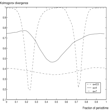
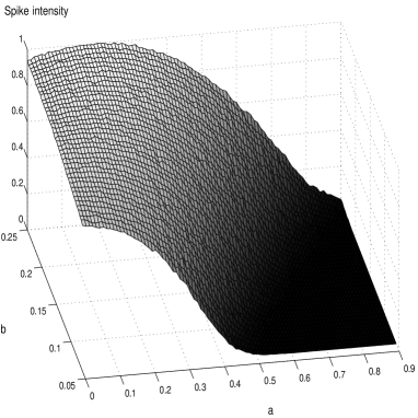
Figure 2: (a) Top: Kolmogorov divergence variation for $q=0.5$ on the output of the model over one period of the signal $s_{t}$ in (5) for three different frequencies and amplitude $A=0.2$. The parameters in the FHN model (1) are $a=0.3$, $b=0.12$, $\delta=1$ and $\varepsilon=0.005$ and the other parameters are $\sigma=100\sqrt{2\cdot 10^{-5}}$, $\lambda=100$, $\alpha=10$, $\beta=100$, $x_{0}=0.25$, $L=1.5$, $R=0.2$, $\tau=50$, $\gamma=0.5$. (b) Bottom: Spontaneous activity (no input signal applied) for the FHN-model, for different values of the parameters $a$ and $b$ and with the other parameters set to $\delta=1$, $\varepsilon=0.005$, $\sigma=100\sqrt{2\cdot 10^{-5}}$ and $\lambda=100$.

based on the assumption that there are enough channels to cover a sufficiently dense set of the phase interval $[0,2\pi)$. It turns out that for high frequencies the $\phi$-divergences do not vary appreciably over a period but in the medium and low frequency cases there will typically be one or two regions of phase values where the divergences are significantly lower, as illustrated in Fig. 2a. However, since the regions where the $\phi$-divergences deviate significantly from their average values generally are relatively small we argue that average divergences as in (8) are relevant as measures of system performance.

Finally we remark that even though the more general “infinite dimensional” formulas for divergences mentioned above in principle could be applied if we generalized the problem to the case where output over a whole time interval $[0,T]$ was observed (instead of only its end point $T$), these formulas are considerably more difficult to handle numerically and involve solving a general nonlinear filtering problem [Liptser and Shiryayev (1977)]. Since the synaptic connection itself represents an averaging over time (and thus “dimensionality reduction” in the problem) we have chosen the approach above as a reasonable compromise to reduce computational complexity while retaining relevance of the model.

2.3 Simulations

The stochastic differential equations were solved using the Euler-Maruyama scheme [Kloeden and Platen (1992)] and the PDFs of the output to the model were estimated using a histogram approach based on counting the number of samples falling in a grid of intervals on the real line. For calculation of the Kolmogorov divergence the so obtained “raw” histograms were sufficient but they proved insufficient for the $\chi^{2}$ and information divergences (which are sensitive to inaccuracies in the representation of the PDFs). Therefore, smoothing with a kernel of the type $e^{-c|x|}$ was applied to the estimated PDFs before the latter two divergences were calculated. In order to reduce the dependence on the smoothing parameter $c$, its values were kept in a region where the results for the Kolmogorov divergence did not vary appreciably depending on weather smoothing was applied or not. Moreover, in this region, the values of the so computed $\chi^{2}$ and information divergences were qualitatively independent of the value of $c$. All our simulations were done using Matlab on UNIX(Digital)/Linux(i386).

3 Results

Our main object of study is the variability of performance, quantified via $\phi$-divergences (cf. Sect. 2.2.2), as a function of parameters. We shall primarily focus on the Kolmogorov divergence, since this is easiest to compute numerically, but we shall also consider performance in terms of the information and $\chi^{2}$ divergences, and deflection ratios.

The regimes of values used for the parameters in the FHN part of the model are chosen on the basis of previous studies [Massanes and Vicente (1999), Alexander et al. (1990)]. First, a nominal set of parameters is chosen for which the FHN output resembles real neuron data and then the parameters are varied around this point. At all times, however, the parameters are kept inside the region where the output is spike-train like i.e., all the resulting FHN outputs are visually similar to the one shown in Fig. 1. The synaptic constants used for the simulation are chosen in order to give realistic EPSP:s for the studied systems and the distance $x_{0}$ is set rather small ($x_{0}=0.25$ on a dendrite of length $L=1.5$) since many synapses in the auditory system, e.g. the endbulb of Held, form connections close to the soma.

3.1 Performance with respect to variation of $a$ and $b$.

A basic example of performance expressed as a function of parameters is shown in Fig. 3a where the Kolmogorov divergence for $A=0.2$, $\omega_{0}=8$, $\delta=1$ and $\sigma=100\sqrt{2\cdot 10^{-5}}$ is displayed as a function of $a$ and $b$. Both $a$ and $b$ have effect on how much excitation that is needed to produce spikes in the FHN output. If $a$ is made smaller the potential barrier height decreases, which gives a larger spike rate. Increasing the value of $b$ has the same effect, since an increase in $b$ can be interpreted as if a bias was added to the input signal. This is illustrated in Fig. 2b where the FHN neuron’s spontaneous activity is displayed for different values of $a$ and $b$.

A marked “ridge” is present in the divergence surface in Fig. 3a, indicating that there is a family of values of the potential parameter $a$ and the bias parameter $b$ that would optimize the ability of the modeled system to detect a (weak) sinusoidal signal. The FHN neurons corresponding to these parameter values have the common property that they fire only sparsely without the signal input but fire with a significant intensity when the signal is present. For parameter values outside the region under the ridge, the Kolmogorov divergence, and associated performance, is uniformly lower. The “plateau” on the left of the ridge is located above parameter values for which the FHN neurons are very easily excited. Given that the spike intensities of the FHN neurons corresponding to these parameter values are roughly independent of the presence or absence of an input signal, the presence of the plateau may seem counterintuitive. However, the firing that takes place when an input signal is applied is much more regular (since it is phase locked to the signal) compared to that taking place when the excitation is just noise. Thus, the divergences corresponding to the systems for which the FHN parts are easily excited are rather large but still clearly smaller than those corresponding to the ridge. In the former region of parameter values it is also possible that an applied input signal decreases the firing rate since the noise-induced firing rate can be larger than the rate given by a phase-locked spike train. Consequently, even though the region of spontaneous firing yields rather large divergences they are are clearly smaller than the divergences on the ridge. The region of low divergences to the right of the ridge is generated by parameter values corresponding to systems of FHN neurons that are very difficult to excite and hardly ever fire, even in the presence of an input signal.

Performing the same type of analysis on the system, but using the $\chi^{2}$ or information divergence instead, yields qualitatively similar results, as seen in Figs. 3b,3c. Due to numerical problems it is hard to calculate the exact height of the ridges, however, and we therefore limit the surfaces’ heights in the figures by truncating values above a certain threshold to the value of the threshold. Even though this prevents a precise estimation of the optimal combinations of parameter values it allows the main objective to be fulfilled; to show the existence of regions with (considerably) better performance in terms of divergences than others. For deflection ratios, on the other hand, the numerical problems are minor, since they can be calculated without explicitly calculating $p_{0}$ and $p_{1}$, which makes DRs more robust. In Fig. 3d DRs for the output of the model are displayed. Also for the DRs a ridge can be seen and the resulting set of optimal values is similar to that for the divergences (though small changes in the position of the ridge can be seen). This qualitative behavior seen in all examples so far, with a (largely) common region of optimal values, is recurrent in all our simulations described in the following.

3.2 Performance for a lower intensity level.

In the previous section we described a simulation which was aimed at investigating optimization of performance as a function of the potential parameter $a$ and the bias parameter $b$, in an otherwise fixed environment. If we change the environment, new values of the parameters will emerge as optimal. For instance, if we lower the intensity level of the noise the location of the ridge appearing in Fig. 3a will change, as seen in Fig. 4a. Together, these two figures illustrate, moreover, that care must be exercised when interpreting results of the stochastic resonance type [Gammaitoni et al. (1998)] for neural processing systems: For a fixed pair of parameters values $a,b$, such as $a=0.6$ and $b=0.12$, the divergence can be higher for a larger noise level but the maximally achievable divergence, obtained on the ridge in the two figures, will be lower. Hence, for a system where adaption to environmental changes is possible, a lower noise intensity is always better in our setting.

3.3 Performance with respect to variation of $a$ and $\delta$.

If we instead of varying the potential parameters $a,b$ vary the relaxation parameter $\delta$ we get the result illustrated in Fig. 4b. Also this divergence surface displays a marked ridge, similar to the one in Fig. 3a, indicating possible combinations of parameter values for best performance.

3.4 Performance for other input signal parameters.

The ridges in the divergence surfaces discussed so far are only relevant for the given input signal and if we change the input by e.g. altering the amplitude or the frequency of the signal we get a different result. Examples of this are shown in Fig. 4c, where the amplitude $A$ is set to 0.1, and in Fig. 4d where the angular frequency $\omega_{0}$ is set to 2. Even though we still can see ridges in both cases they are different in shape than the first one in Fig. 3a. Obviously, the divergence decreases with decreased signal amplitude and the height of the ridge becomes lower in Fig. 4c, but the location of the ridge changes only slightly and it appears as if only a slight change of optimal parameter values occurs. When varying the frequency however, the ridge clearly moves to an entirely new position and new parameter values render optimal performance.

4 Discussion

We have described a method for analyzing the information processing capability in the primary part of the mammalian auditory nervous system using fundamental statistical and information theoretical performance criteria, quantitatively expressed by $\phi$-divergences. Our premise has been that, since these criteria are highly relevant for the processing taking place in this system, the non-existence of well defined global maxima of these criteria occuring in the interior of regions of feasible system parameters would suggest incompleteness or incorrectness of the overall model. (Loosely speaking, one can argue that such global interior maxima must exist for the “right” criteria in a “correct” model since otherwise parameters would have to be set at boundaries in order to achieve optimal behavior. Parameters at boundaries would favor structural change by evolution until only interior optima occur, whereby the “drive” for structural change ceases). One instance of this point is that without taking into account the synaptic plasticity, it can be shown that the divergence surfaces will have a qualitatively different shape, with an additional ridge that, at least partly, will yield optimal parameter values that are unphysical. However, the observed “ridges” in the divergence and deflection surfaces in Figs. 3,4 indeed allow for optimization of performance by taking parameter values in the interior of the domain of values that have physical significance. Since the model is based on fairly standard and well accepted components (e.g. the FHN model), which we feel capture the essential mechanisms involved in the information processing considered here, we believe that the results in fact can be interpreted as a quantitative indication of how some of the parameters in the auditory system presumably must be set. In particular this applies to the quiescent firing rate (QFR) which, in real systems under this assumption, must take values (as a result of evolution) near those that correspond to the maxima of the performance measures considered here. Verifying this is a topic for further research, however.

The conclusion about the QFR is based on the qualitative observation that all the “ridges” appearing in the divergence and deflection surfaces correspond to parameter values that lie a certain “thin” or “manifold like” set in parameter space. A closer examination of this set shows that the combinations of parameter values that correspond to e.g. the ridge in Fig. 3a describe systems that have virtually the same firing intensity in the absence of an external signal, i.e. virtually the same QFR. Since this specific QFR also is common for all optimal values of parameter combinations corresponding to the ridges in Figs. 4a,4b, and in all other simulations that we have tried with the same input signal, this strongly suggests a connection between the QFR and the information processing performance of the system. Further evidence supporting this hypothesis can be seen in Figs. 4c,4d which show that the optimal QFR, and thereby the optimal set of parameters, is very little affected by a change in our (weak) signal amplitude but changes considerably with the applied frequency. This reflects well the frequency division of sound performed in the inner ear, as discussed in Section 2.2. A more detailed investigation of the frequency dependence also shows that the optimal QFR in our model increases with increasing frequency. Even though existing real data is inconclusive on this point, Kiang’s classical data [Kiang (1965)] can be interpreted to support the hypothesis that such a frequency dependence exists. However, experiments are needed to resolve the issue. Finally we point out that even though the location of the ridge in e.g. Figs. 3a,3b,3c is largely the same it does vary slightly depending on which divergence or deflection is considered, which is to be expected since these performance measures are not identical. In particular, the $\chi^{2}$-divergence in Fig. 3b can, as explained in Sec. 2.2.1, be considered to be a first order approximation of the information divergence in Fig. 3c.

All constants in our model have been chosen in order to produce as realistic data as possible. The choices are not critical though, since in most of the simulations where the values of the constants are varied (in a reasonable large interval) the results are qualitatively invariant. Our approach therefore offers a new qualitative, and possibly also a quantitative, explanation of the different levels of QFRs observed in the auditory nerve.

5 Acknowledgements

The authors would like to acknowledge fruitful discussions with Prof. A. Longtin of Ottawa Univ. which led to improvement of the results in several aspects and to Dr. A. Bulsara of SPAWAR SSC, San Diego, CA, for many insightful suggestions which clarified the presentation of the material. MFK would also like to thank Prof. Longtin for his hospitality during a visit in Ottawa.

6 Figures

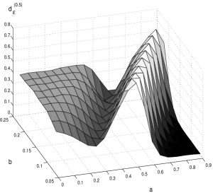
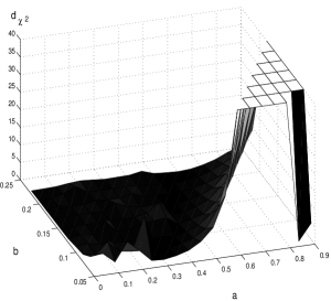
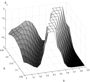
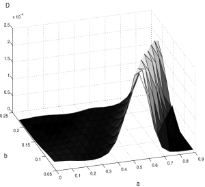
Figure 3: (a) Top left: The Kolmogorov divergence for $\delta=1$, $\varepsilon=0.005$, $A=0.2$, $\omega_{0}=8$, $\sigma=100\sqrt{2\cdot 10^{-5}}$, $\lambda=100$, $\alpha=10$, $\beta=100$, $x_{0}=0.25$, $L=1.5$, $R=0.2$, $\tau=50$, $\gamma=0.5$, $q=0.5$ and different values of the potential parameter $a$ and the bias parameter $b$. (b) Top right: The $\chi^{2}$ divergence for different values of the potential parameter $a$ and the bias parameter $b$ when the other parameter values are the same as in Fig 3a. Due to the unreliability for high values of the divergence no value above 40 has been plotted. (Eventually the $\chi^{2}$-divergence decreases to zero, when $a$ becomes sufficiently large, since then there will be almost no spikes generated.) (c) Bottom left: The information divergence for different values of the potential parameter $a$ and the bias parameter $b$ when the other parameter values are the same as in Fig 3a. Due to the unreliability for high values of the divergence no value above 3 has been plotted. (d) Bottom right: The deflection ratio for different values of the potential parameter $a$ and the bias parameter $b$ when the other parameter values are the same as in Fig 3a.

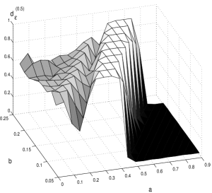
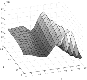
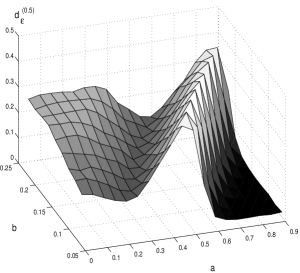
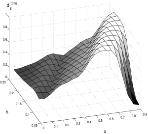
Figure 4: (a) Top left: The Kolmogorov divergence for different values of the potential parameter $a$ and the bias parameter $b$, when the other parameter values are the same as in Fig 3a except for the noise intensity, which is lower ($\sigma=100\sqrt{2\cdot 10^{-6}}$). (b) Top right: The Kolmogorov divergence for different values of the potential parameter $a$ and the relaxation parameter $\delta$ for $b=0.12$ and with the other parameter values as in Fig 3a. (c) Bottom left: The Kolmogorov divergence for different values of the potential parameter $a$ and the bias parameter $b$ when the other parameter values are the same as in Fig 3a except for the signal amplitude, which is lower ($A=0.1$). (d) Bottom right: The Kolmogorov divergence for different values of the potential parameter $a$ and the bias parameter $b$ when the other parameter values are the same as in Fig 3a except for the frequency, which is lower ($\omega_{0}=2$).

References

- Alexander et al. (1990) J.C. Alexander, E.J. Doedel and H.G. Othmer (1990) On the Resonance Structure in a Forced Excitable System. SIAM J. Appl. Math. 50:1373–1418.
- Ali and Silvey (1966) S. Ali and D. Silvey (1966) A General Class of Coefficients of Divergence of One Distribution from Another. J. Roy. Stat. Soc. B28:131–142.
- Basseville (1989) M. Basseville (1989) Distance Measures for Signal Processing and Pattern Recognition. Signal Processing. 18:349–369.
- Camalet et al. (2000) S. Camalet, T. Duke, F. Jülicher and J. Prost (2000) Auditory Sensitivity Provided by Self-Tuned Critical Oscillation of Hair Cells. Proc. Nat. Acad. Sci. 97:3183–3188.
- Cover and Thomas (1991) T.M. Cover and J.A. Thomas (1991) Elements of Information Theory. Wiley, New York, NY.
- Eguíluz et al. (2000) V.M. Eguíluz, M. Ospek, Y. Choe, A.J. Hudspeth and M.O. Magnasco (2000) Essential Nonlinearities in Hearing. Phys. Rev. Lett. 84:5232–5235.
- FitzHugh (1961) R.A. FitzHugh (1961) Impulses and Physiological States in Theoretical Models of Nerve Membrane. BioPhys. J. 1:445–466.
- Gammaitoni et al. (1998) L. Gammaitoni, P. Hänggi, P. Jung and F. Marchesoni (1998) Stochastic Resonance. Rev. Mod. Phys. 70:223–287.
- Geisler (1998) C.D. Geisler (1998) From Sound to Synapse: Physiology of the Mammalian Ear, Oxford University Press, New York, NY.
- Gerstner and Van Hemmen (1992) W. Gerstner and J.L. Van Hemmen (1992) Associative Memory in a Network of “Spiking” Neurons. Network. 3:139–164.
- Jack and Redman (1971) J.J.B. Jack and S.J. Redman (1971) The Propagation of Transient Potentials in some Linear Cable Structures. J. Physiol. 215:283–320.
- Kiang (1965) N. Kiang (1965) Discharge Patterns of Single Fibers in the Cat’s Auditory Nerve. M.I.T. Press, Cambridge, Massachusetts.
- Kistler and Van Hemmen (1999) W.M. Kistler and J.L. Van Hemmen (1999) Short-Term Plasticity and Network Behavior. Neural Comp. 11:1579–1594.
- Kloeden and Platen (1992) P.E. Kloeden and E. Platen (1992) Numerical Solution of Stochastic Differential Equations. Springer, Berlin.
- Koch (1999) C. Koch (1999) Biophysics of Computation: Information Processing in Single Neurons, Oxford University Press, New York.
- Liese and Vajda (1987) F. Liese and I. Vajda (1987) Convex Statistical Distances. Teubner, Leipzig.
- Liptser and Shiryayev (1977) R.S. Liptser and A.N. Shiryayev (1977) Statistics of Random Processes I General Theory: Springer, New York.
- Longtin (1993) A. Longtin (1993) Stochastic Resonance in Neuron Models. J. Stat. Phys. 70:309–327.
- Manwani and Koch (1999) A. Manwani and C. Koch (1999) Detecting and Estimating Signals in Noisy Cable Structures, II: Information Theoretical Analysis. Neural Comp. 11:1831–1873.
- Massanes and Vicente (1999) S.R. Massanes and C.J.P. Vicente (1999) Nonadiabatic Resonances in a Noisy Fitzhugh-Nagumo Neuron Model. Phys. Rev. E. 59:4490–4497.
- Nagumo et al. (1962) J.S. Nagumo, S. Arimoto and S. Yoshizawa (1962) An Active Pulse Transmission Line Simulating Nerve Axon. Proc. IRE. 50:2061–2070.
- Robinson et al. (2000) J.W.C. Robinson, J. Rung, A.R. Bulsara and M.E. Inchiosa (2000) General Measures for Signal-Noise Separation in Nonlinear Systems, to appear in Phys. Rev. E.
- Rung and Robinson (2000) J. Rung and J.W.C. Robinson (2000) A Statistical Framework for the Description of Stochastic Resonance Phenomena. In: D.S. Broomhead, E.A. Luchinskaya, P.V.E. McClintock, and T. Mullin, eds. STOCHAOS, Stochastic and Chaotic Dynamics in the Lakes. American Institute of Physics, Melville, NY.
- Salicru (1993) M. Salicrú (1993) Connections of Generalized Divergence Measures with Fisher Information Matrix. Information Sciences. 72:251–269.
- Scott (1975) A.C. Scott (1975) The Electrophysics of a Nerve Fiber. Rev. Mod. Phys. 47:487–533.
- Stemmler (1996) M. Stemmler (1996) A Single Spike Suffices: the Simplest Form of Stochastic Resonance in Model Neurons. Network: Computation in Neural Systems. 7:687–716.
- Tsodyks and Markham (1997) M.V. Tsodyks and H. Markham (1997) The Neural Code Between Neocortical Pramidal Neurons Depends on Neurotransmitter Release Probability. Proc. Natl. Acad. Sci. 94:719–723. (See also correction at http://www.pnas.org)
- Tuckwell (1988) H.C. Tuckwell (1988) Introduction to Theoretical Neurobiology. Cambridge University Press, Cambridge.
- Webster et al. (1992) D.B. Webster, A.N. Popper and R.R. Fay, eds. (1992) The Mammalian Auditory Pathway: Neuroanatomy, Springer, Ney York, NY.
- Zador (1998) A. Zador (1998) Impact of the Unreliability on the Information Transmitted by Spiking Neurons. J. Neurophysiol. 79:1219–1229.