Slow light in moving media

Abstract

We review the theory of light propagation in moving media with extremely low group velocity. We intend to clarify the most elementary features of monochromatic slow light in a moving medium and, whenever possible, to give an instructive simplified picture.

1 Introduction

Waves experience moving media as effective gravitational fields. To understand why, imagine a definite example — light traveling in a moving transparent fluid such as flowing water [1, 2]. In each drop of the liquid, light propagates along a straight line and so each drop distinguishes a particular inertial frame. Now imagine light passing from one drop to a next one which happens to move with a different velocity vector. Again, the new drop in the way of the light distinguishes an inertial frame, but this new frame will differ from the previous one. Light traveling in a non–uniformly moving medium is constantly forced to adapt to new inertial frames. An analogous situation occurs in curved space–time when light, and all other matter, experiences space and time as consisting of connected inertial frames. Space–time can be thought as being locally flat, even in the vicinity of the most violent gravitating objects, yet each local frame is non-trivially connected to the neighboring frames, a connection mathematically described in terms of the curvature tensor [3]. In a moving medium, the local co-moving frames of the medium play the role of the local pieces of flat space–time. Because theses pieces differ in non–uniform flows, light propagation in a moving medium resembles light propagation in curved space–time, i.e. the medium appears to light as an effective gravitational field [4]-[6].

One could conceive of employing moving media for creating artificial astronomical objects in the laboratory. For example, water going down the drain of a bathtub appears to light as a rotating black hole. However, in order to observe spectacular effects of general relativity in laboratory–based analogues, truly astronomical flow velocities are required. For establishing a black hole, the fluid should move faster than the speed of light in the medium ($c$ divided by the refractive index $n$). The chances of creating analagoes of black holes are much better when one employs sound instead of light in appropriate supersonic flows [7]-[16]. One of the most fascinating effects of black holes is Hawking radiation [17]-[19], the spontaneous generation of photon pairs near the hole’s horizon where one of the photons falls into the hole and the other tunnels out of the attraction zone and become visible. The acoustical equivalent of Hawking radiation is quantum sound in superfluids [7]-[16]. However, superfluidity tends to break down before the fluid has a chance to move faster than the speed of sound [20]. Furthermore, quantum sound and flow are just two aspects of the same object, the quantum liquid. The flow is the macroscopic and the sound the microscopic motion. Under extreme circumstances such as near the horizon of a sonic black hole, a clear distinction between sound and flow might be difficult. An advantage of light in a moving medium is the clear separation between wave and flow, and both light and medium can be regarded as separate quantum systems.

Recently, light has been slowed down dramatically [21]-[23] due to an effect called Electromagnetically Induced Transparency [24]-[26]. The use of slow light could open the opportunity for observing the radiation of quantum–optical black holes. Note, however, that slow light is a more complicated phenomenon than light in a moving non–dispersive dielectric where the refractive index does not depend on the frequency of light. Slow light is based on a highly dispersive medium created by dressing the atoms of the medium with an appropriate light beam. Instead of the phase velocity only the group velocity is reduced. Therefore, it is not always advisable to conclude directly from the behavior of light in ordinary dielectrics to the motional effects of slow–light media. It is the purpose of these notes to clarify the most elementary features of slow light in a moving medium [27] and, whenever possible, to give an instructive simplified picture.

2 Dispersion relation

Imagine the medium as being decomposed into drops. Each drop should be small enough such that the flow does not vary significantly within the size of the drop, but each drop should be sufficiently large to sustain several optical oscillations. We thus assume that the wave length of light is much shorter than the typical scale of changes in the flow. In this case, we can describe light by a dispersion relation in the local co–moving frame of each medium drop denoted with primes

$$k^{\prime 2}-\frac{\omega^{\prime 2}}{c^{2}}-\chi(\omega^{\prime})\,\frac{\omega^{\prime 2}}{c^{2}}=0\,\,.$$ (1)

The susceptibility $\chi(\omega^{\prime})$ characterizes the medium. In Electromagnetically Induced Transparency [24]-[26] a coupling beam dresses the upper two levels of a three–level atom shown schematically in Fig. 1.

Figure 1: Three level system needed for the creation of electromagnetically induced transparency. A strong drive laser field couples the levels a and c, making the medium transparent for the weak probe laser tuned to the transition a$\leftrightarrow$b.

The dressing of the upper two levels influences strongly the propagation of the probe light with a frequency that should match the atomic transition frequency $\omega_{0}$ between the lower and one of the upper levels. Exactly on resonance, the medium decouples from the probe light and becomes transparent, whereas ordinary dielectrics are extremely absorbing at atom–light resonances. Furthermore, the susceptibility changes rapidly, see Fig. 2,

Figure 2: Susceptibility for the probe laser beam in electromagnetically induced transparency. The plot shows the dependence of the real (whole lines) and imaginary (dashed lines) parts of the susceptibility $\chi$ on the detuning $\Delta$ of the probe beam. The drive beam is assumed to be on resonance. Arbitrary units are used.

and, near the resonance, $\chi(\omega^{\prime})$ assumes a linear dependence on the detuning between the light frequency $\omega^{\prime}$ and the atomic frequency $\omega_{0}$,

$$\chi(\omega^{\prime})=\frac{2c}{\omega_{0}v_{g}}\,(\omega^{\prime}-\omega_{0})\,\,,$$ (2)

giving rise to a very low group velocity $v_{g}$. If the slow–light medium is moving coherently, the motion will slightly detune each atom from exact resonance due to the Doppler effect.

Figure 3: Slow light in moving media. The medium should move orthogonally to the coupling beam (grey arrow). This beam prepares the medium such that the group velocity of light is significantly reduced. The probe beam (lines) experiences the Doppler detuning due to the moving medium and becomes deflected or even trapped.

Imagine that the flow of the medium, ${\bf u}$, varies only in two dimensions and that the coupling beam propagates orthogonally to the flow, see Fig 3. In this case we can ignore the first–order Doppler effect of the coupling beam and we should focus only on the Doppler detuning of the probe. In the laboratory frame the probe shall be monochromatic at the atomic frequency $\omega_{0}$. In the co–moving local frames of the medium the probe–light frequency is Doppler–shifted with the detuning

$$\omega^{\prime}-\omega_{0}=-{\bf u}\cdot{\bf k}\,\,,$$ (3)

to first order in $u/c$. Let us transform the dispersion relation (1) to the laboratory frame. We take advantage of the Lorentz invariance of $k^{2}-(\omega/c)^{2}$ and obtain to first order in $u/c$ the relation

$$k^{2}-k_{0}^{2}+2\,\frac{k_{0}}{v_{g}}\,{\bf u}\cdot{\bf k}=0$$ (4)

with

$$k_{0}=\frac{\omega_{0}}{c}\,\,.$$ (5)

In Ref. [27] a more complicated dispersion relation has been derived which is correct up to second order in $u/c$. Note that the relation (4) describes effects in leading order of $u/(v_{g}c)^{1/2}$, because the second–order corrections of Ref. [27] are proportional to $v_{g}^{-1}$.

3 Magnetic model and metric

We are going to use the simplified relation (4) to illuminate the most characteristic features of slow light in moving media. First we note that we can write the relation as

$$\left({\bf k}+k_{0}\,\frac{\bf u}{v_{g}}\right)^{2}-k_{0}^{2}\frac{u^{2}}{v_{g}^{2}}=k_{0}^{2}\,\,.$$ (6)

Monochromatic light waves with fixed polarization thus obey the wave equation

$$\left(-i\nabla+k_{0}\,\frac{\bf u}{v_{g}}\right)^{2}\phi-k_{0}^{2}\frac{u^{2}}{v_{g}^{2}}\,\phi=k_{0}^{2}\,\phi\,\,.$$ (7)

The flow has a two–fold effect: On one hand, the velocity ${\bf u}$ appears as an effective vector potential, for example the magnetic vector potential acting on an electron wave [28], and, on the other hand, the hydrodynamic pressure proportional to $u^{2}$ [29] acts as a scalar potential. This resembles the Röntgen effect of static electromagnetic fields on polarizable atoms [30, 31].

Alternatively, we can regard the flow as generating an effective gravitational field. To see this, we introduce the four–dimensional wave vector

$$k_{\nu}=(k_{0},-{\bf k})\,\,,$$ (8)

and, adopting Einstein’s summation convention, write the dispersion relation (4) as

$$g^{\mu\nu}k_{\mu}k_{\nu}=0$$ (9)

with the contravariant metric tensor

$$g^{\mu\nu}=\left(\begin{array}[]{cc}1&{\displaystyle{\bf u}/{v_{g}}}\\ {\displaystyle{\bf u}/{v_{g}}}&-{\bf 1}\end{array}\right)\,\,.$$ (10)

Four–dimensional wave vectors are null vectors with respect to the effective metric $g^{\mu\nu}$ and, in turn [1], light rays follow zero-geodesics with respect to the line element

$$ds^{2}=g_{\mu\nu}dx^{\mu}dx^{\nu}\quad,\quad dx^{\nu}=(ct,{\bf x})\,\,.$$ (11)

The covariant metric tensor $g_{\mu\nu}$ is the inverse of the contravariant one, and is given by

$$g_{\mu\nu}=\frac{1}{1+{u^{2}}/{v_{g}^{2}}}\left(\begin{array}[]{cc}1&{\displaystyle{\bf u}/{v_{g}}}\\ {\displaystyle{\bf u}/{v_{g}}}&-{\bf 1}\end{array}\right)\,\,.$$ (12)

In contrast to sound [14] or light in non–dispersive media [1], a genuine event horizon of slow light cannot exist at this level of approximation. The potential existence of an event horizon is thus confined to effects to second order in $u/(v_{g}c)^{1/2}$which are excluded from our simplified model [32].

4 Non–relativistic analogue

To get more insight into the behavior of slow light in moving media, let us study another analogue. Consider a non–relativistic free particle attached to moving frames. The particle is supposed to move freely in each of the local frames but is bound to adapt from one frame to the next, similar to light in drops of flowing water. However we use pure non–relativistic physics to transform from frame to frame. In case the local frames constitute a global frame, for example a rotating solid body, the particle would move along a straight line with respect to this frame. In the laboratory frame, the particle’s trajectory appears to be bent, attributed to the effect of Coriolis and centrifugal forces. The Lagrange function of such a fictitious non–relativistic particle is

$$L=\frac{1}{2}\,{v^{\prime}}^{2}=\frac{1}{2}\,({\bf v}-{\bf w})^{2}\,\,,$$ (13)

up to a constant mass factor that we can set to unity, because we are interested in inertial effects only. The velocity of the local intertial frames is ${\bf w}$ and we have used the non–relativistic addition theorem of velocities

$${\bf v}^{\prime}={\bf v}-{\bf w}\,\,.$$ (14)

Note that we could apply Einstein’s relativistic addition theorem of velocities to describe light in moving non–dispersive media of refractive index $n$, but we should use an effective speed of light of $c/n$ in the theorem. The momentum of the fictitious non–relativistic particle is

$${\bf p}\equiv\frac{\partial L}{\partial{\bf v}}={\bf v}-{\bf w}$$ (15)

and the Hamiltonian is

$$H\equiv{\bf v}\cdot{\bf p}-L=\frac{1}{2}\,p^{2}-{\bf w}\cdot{\bf p}=E\,\,.$$ (16)

The important point is that we can translate the Hamiltonian (16) into the dispersion relation (4) by setting

$${\bf p}=c\,\frac{\bf k}{k_{0}}\,\,,\quad{\bf w}=\frac{c}{v_{g}}\,{\bf u}\,\,,\quad E=\frac{1}{2}\,c^{2}\,\,.$$ (17)

with the enhanced effective frame velocity ${\bf w}$ [33]. Consequently, slow light experiences the moving medium in the same way as a non–relativistic particle experiences moving inertial frames. Excused by its fictitious nature, the “non–relativistic” particle would move at an extraordinary speed reaching $c$ in regions where the medium is at rest, because the energy is

$$\frac{1}{2}\,c^{2}=E=H=\frac{1}{2}\,v^{2}-\frac{1}{2}\,w^{2}\,\,.$$ (18)

We obtain from Hamilton’s equations,

$${\bf v}=\dot{\bf r}=\frac{\partial H}{\partial{\bf p}}\,\,,\quad\dot{\bf p}=-\frac{\partial H}{\partial{\bf r}}\,\,,$$ (19)

the equation of motion of the fictitious particle

$$\dot{\bf v}=(\nabla\times{\bf w})\times{\bf v}+\frac{1}{2}\,\nabla w^{2}\,\,.$$ (20)

The first term describes the Coriolis and the second the centrifugal force.

5 Light rays around a vortex

Consider a specific example of a non–uniform flow, a vortex. Quantum vortices in alkali Bose–Einstein condensates have been recently made [34, 35]. They give rise to intriguing slow-light phenomena. However, vortices do not posses genuine event horizons [32] and they will not radiate spontaneously. The flow of an ideal vortex of vorticity ${\cal W}$ is

$${\bf u}=\frac{\cal W}{r}\,{\bf e}_{\varphi}=i\,\frac{\cal W}{z^{*}}\,\,,$$ (21)

written in polar coordinates or using the complex notation $z=x+iy$, $z^{*}=x-iy$ of the planar Cartesian coordinates $x,y$. The curl of the vortex flow vanishes,

$$\nabla\times{\bf u}={\bf 0}\,\,,$$ (22)

and hence we obtain the equation of motion of a particle in an attractive $r^{-2}$ potential [36]-[38],

$$\dot{\bf v}=\frac{1}{2}\,\nabla w^{2}=-\,\frac{c^{2}{\cal W}^{2}}{v_{g}^{2}}\,\frac{\bf r}{r^{4}}\,\,,$$ (23)

or, in complex notation,

$$\ddot{z}+\frac{c^{2}{\cal W}^{2}}{v_{g}^{2}}\,\frac{z}{|z|^{4}}=0\,\,.$$ (24)

The trajectories of the fall into a $r^{-2}$ singularity are well known in polar coordinates [36] but here we suggest a more elegant description using the complex notation of the planar Cartesian coordinates,

$$z=\left(-ct+i\,\frac{b}{\mu}\right)^{(1+\mu)/2}\left(-ct-i\,\frac{b}{\mu}\right)^{(1-\mu)/2}$$ (25)

with the real parameter $b$ and

$$\mu=\left(1-\frac{{\cal W}^{2}}{v_{g}^{2}b^{2}}\right)^{-1/2}\,\,.$$ (26)

One can easily verify that this solution satisfies the equation of motion (24). In the infinite past, $t\rightarrow-\infty$, the trajectories approach

$$z\sim-ct+ib\,\,.$$ (27)

From this asymptotics we see that the light is incident from the right to the left with initial velocity $c$ and impact parameter $b$. Depending on the impact parameter, the coefficient $\mu$ is real or purely imaginary. In the case of a real $\mu$ when ${\cal W}^{2}<v_{g}^{2}b^{2}$ the incident light particle will be able to escape, because the modulus squared of $z$, $c^{2}t^{2}+b^{2}/\mu^{2}$, will never reach zero, the vortex core. In the infinite future, $t\rightarrow+\infty$, the particle will approach

$$z\sim ct\,(-1)^{\mu}+ib=cte^{i\pi\mu}+ib$$ (28)

and, consequently, leaves at the angle $\pi\mu$. In the case of a purely imaginary coefficient $\mu$ when ${\cal W}^{2}>v_{g}^{2}b^{2}$ the light is sucked into the vortex, because the modulus squared of $z$, $c^{2}t^{2}+b^{2}/\mu^{2}$, reaches zero at the time $t=-|b/(\mu c)|$. In practice, the light will hit the vortex core and will bounce back. In theory, the fictitious light particle disappears from this world and reappears on another Riemann sheet. In the borderline case when ${\cal W}^{2}=v_{g}^{2}b^{2}$ the parameter $\mu$ tends to infinity and the trajectory approaches

$$z=-ct\lim_{\mu\rightarrow\infty}\left(1-\frac{1}{\mu}\,\frac{ib}{ct}\right)^{\mu}=-ct\,\exp\left(-\frac{ib}{ct}\right)=\exp\left(\pm\frac{i{\cal W}}{v_{g}ct}\right)\,\,.$$ (29)

Light falling into the vortex core describes distinctive spirals illustrated in Fig. 4.

Figure 4: Light rays spiraling towards the vortex core. The plot shows the limiting spiral of described in Eq. (29).

Light waves around a vortex

Near the vortex core, rays of slow light feel the presence of the centrifugal $r^{-2}$ attraction but no Coriolis force, because the curl of the flow vanishes. Light waves, however, will show a distinctive interference pattern, an optical Aharonov–Bohm effect [39]-[42] due to the long–range nature of a vortex flow. Far outside the vortex core, light rays are hardly deflected, yet rays passing the vortex in flow direction will be dragged and those swimming against the current lag behind. This does not affect the ray trajectories but it produces a phase shift between the dragged and the lagging rays, and, in turn, creates a typical interference pattern [41, 42]. Note that the Aharonov–Bohm effect of waves in moving media is not restricted to light. Indeed, Berry et al. [43] have reported and analyzed a beautiful bathtub experiment with water waves in a tank, visualizing clearly the interference structure generated by the Aharonov-Bohm effect. A further experiment has been reported [44] showing spiral waves. Acoustical analogues of the effect have been observed in moving classical media [45] and are predicted for superfluids [46]. The acoustical effect might even lead to a friction felt by traveling vortices due to the so-called Iordanskii force [47]-[49]. The optical Aharonov–Bohm effect of slow light [27] can be applied to observe in situ the flow of quantum vortices in alkali Bose–Einstein condensates [34, 35] using phase–contrast imaging [50].

Consider the propagation of slow–light waves through a vortex flow. In polar coordinates the wave equation (7) is

$$\left[\frac{\partial^{2}}{\partial r^{2}}+\frac{1}{r}\frac{\partial}{\partial r}+\frac{1}{r^{2}}\left(\frac{\partial}{\partial\varphi}+i\nu_{AB}\right)^{2}+\frac{\nu_{AB}^{2}}{r^{2}}\right]\phi=k_{0}^{2}\,\phi$$ (30)

with the optical Aharonov–Bohm flux quantum

$$\nu_{AB}=k_{0}\,\frac{\cal W}{v_{g}}\,\,.$$ (31)

We could simply eliminate the optical analogue of the vector potential by representing $\phi$ as

$$\phi=\phi_{0}\,\exp(-i\nu_{AB}\varphi)$$ (32)

where $\phi_{0}$ feels only the local $r^{-2}$ attraction due to the centrifugal force. The modulation $\exp(-i\nu_{AB}\varphi)$ describes the long–range Aharonov–Bohm phase pattern [41]. Strictly speaking, however, the ansatz (32) is only justified when the function $\exp(-i\nu_{AB}\varphi)$ is single–valued after a complete cycle of $\varphi$, i.e. when $\nu_{AB}$ is an integer. For non–integer flux quanta the interference pattern is slightly more complicated, showing, most prominently, a line of zeros of the wave function after passing the vortex (which resolves the problem of a multi–valued phase, because a phase is not defined when the amplitude is zero). Even in the case of non–integer optical flux quanta $\nu_{AB}$, the modulation $\exp(-i\nu_{AB}\varphi)$ accounts for the dominant phase pattern.

The correct positive–frequency component of a slow–light wave incident from the right is an appropriate superposition [31]

$$\phi=\sum_{m=-\infty}^{+\infty}\phi_{m}$$ (33)

of the partial waves

$$\phi_{m}=u_{m}(r)\,\exp(im\varphi-i\omega_{0}t)\,\,,\quad u_{m}=(-i)^{\nu}\,J_{\nu}(k_{0}r)$$ (34)

characterized by the Bessel functions $J_{\nu}$ with the index

$$\nu=\sqrt{(m+\nu_{AB})^{2}-\nu_{AB}^{2}}\,\,.$$ (35)

Figure 5 shows plots of slow–light waves around a vortex to illustrate the long–range phase shift brought about by the optical Aharonov–Bohm effect.

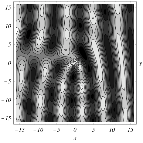
Figure 5: Slow-light waves traveling through a vortex. The dragging effect of the vortex shifts the phase of the incident light, depending on whether the light propagates with or against the flow.

Close to the vortex core, a light ray is doomed to fall into the singularity when the square of the impact parameters, $b^{2}$, does not exceed ${\cal W}^{2}/v_{g}^{2}$. In this case the angular momentum $m$ lies in the interval

$$-2\nu_{AB}\leq m\leq 0\,\,,$$ (36)

because, according to Eqs. (15,17) and the pattern (21) of the vortex flow,

$${\bf r}\times{\bf k}={\bf r}\times k_{0}({\bf v}-{\bf w})/c=(k_{0}b-\nu_{AB})\,{\bf e}_{z}\,\,.$$ (37)

The fall of light rays into the vortex core corresponds to a drastic change of the behavior of the corresponding partial waves $\phi_{m}$. In the case (36) the index (35) of the Bessel function in a radial wave (34) is purely imaginary. Using the first term in the power–series expansion of the Bessel functions [51] we see that $u_{m}$ is rapidly oscillating near the core,

$$u_{m}\sim\frac{(-i)^{\nu}}{\Gamma(\nu+1)}\,\left(\frac{k_{0}r}{2}\right)^{\nu}=\frac{(-i)^{\nu}}{\Gamma(\nu+1)}\,\exp\left[i{\rm Im}\,\nu\,\ln\left(\frac{k_{0}r}{2}\right)\right]\,\,.$$ (38)

This describes a rapid flow of light towards the centre of attraction, if ${\rm Im}\,\nu$ is negative and an outgoing wave for the positive branch. Far outside the vortex core, $r\rightarrow\infty$, the radial waves approach

$$u_{m}\sim\frac{1}{\sqrt{2\pi k_{0}r}}\,\left[\exp\left(ik_{0}r-i\pi\nu-i\frac{\pi}{4}\right)+\exp\left(-ik_{0}r+i\frac{\pi}{4}\right)\right]\,\,,$$ (39)

as we see from the asymptotics of the Bessel functions [51]. For a negative imaginary $\nu$ the second term in Eq. (39) dominates and so most of the light is incident, yet a small fraction with weight $\exp(-2i\pi\nu)$ is able to tunnel out of the attraction zone.

Where is the borderline between pure influx and partial tunneling out of the attraction zone? Consider the geometrical optics of a radial wave. We make the eikonal ansatz

$$u_{m}=c_{m}^{+}u_{m}^{+}+c_{m}^{-}u_{m}^{-}\,\,\quad u_{m}^{\pm}=|u_{m}|\,\exp(\pm iR)\,\,,$$ (40)

regard $|u_{m}|$ as a slowly varying envelope, and obtain from the wave equation (30) the radial eikonal

$$R=i\nu\left[\sqrt{\rho^{2}+1}-{\rm arsinh}\left(\frac{1}{\rho}\right)+i\frac{\pi}{2}\right]\,\,,\quad\rho=\frac{k_{0}r}{i\nu}\,\,.$$ (41)

Quite typically, valuable insight into the behavior of waves can be gained by analytical continuation to the complex plane of the wave’s argument. Consider the line in the complex plane of the radius $r$ where the eikonal is purely imaginary, i.e. where

$${\rm Re}\,\left[\sqrt{\rho^{2}+1}-{\rm arsinh}\left(\frac{1}{\rho}\right)\right]=0\,\,,$$ (42)

see Fig. 6. This line is called a Stokes line [52, 53]. When passing a Stokes line, one component of the superposition (40) becomes exponentially small and hence irrelevant [52]. The asymptotics in the limit of geometrical optics switches from a two–component regime, for example in–and–out flux, to a single component behavior, such as pure influx [52]. The Stokes line in Fig. 6 thus marks the boundary where light is able to tunnel out of the optical black hole.

Figure 6: Stokes lines of an optical black hole. Stokes lines [52] are lines in the complex plane of the radius $r$ where the radial eikonal of light waves is purely imaginary. The lines connect the turning points of light rays which are complex in the general case of trapping (and purely imaginary for an optical black hole). The Stokes lines are calculated from the radial part of the eikonal (41) and are displayed in the scaled units employed there. The arrows indicate the light flux in the regions bounded by a Stokes line.

6 Summary

We analyzed the propagation of slow light in moving media in the case when the light is monochromatic in the laboratory frame. Slow light is generated by the electromagnetically induced transparency of an atomic transition. The Doppler detuning due to the moving medium generates flow-dependent effects. We considered analogies to magnetism and general relativity and studied light propagation around a vortex in some detail. The subject is far from being exhausted — light detuned from the atomic resonance and non–monochromatic light will behave differently, opening perhaps new exciting analogies and opportunities for laboratory tests of astronomical effects on Earth.

7 Acknowledgements

U.L. acknowledges the support of the Alexander von Humboldt Foundation and of the Göran Gustafsson Stiftelse during his stay at the Royal Institute of Technology. P.P. was partially supported by the research consortium Quantum Gases of the Deutsche Forschungsgemeinschaft.

References

- [1] U. Leonhardt and P. Piwnicki, Phys. Rev. A 60, 4301 (1999).
- [2] U. Leonhardt and P. Piwnicki, Light in moving media, Contemp. Phys. (in press).
- [3] L. D. Landau and E. M. Lifshitz, The Classical Theory of Fields (Pergamon, Oxford, 1975).
- [4] W. Gordon, Ann. Phys. (Leipzig) 72, 421 (1923).
- [5] Pham Mau Quan, C. R. Acad. Sci. (Paris) 242, 465 (1956).
- [6] Pham Mau Quan, Archive for Rational Mechanics and Analysis 1, 54 (1957/58).
- [7] W. G. Unruh, Phys. Rev. Lett. 46, 1351 (1981).
- [8] W. G. Unruh, Phys. Rev. D 51, 2827 (1995).
- [9] T. A. Jacobson, Phys. Rev. D 44, 1731 (1991).
- [10] T. A. Jacobson and G. E. Volovik, Phys. Rev. D 58, 064021 (1998).
- [11] N. B. Kopnin and G. E. Volovik, JETP Lett. 67, 140 (1998).
- [12] T. A. Jacobson and G. E. Volovik, JETP Lett. 68, 874 (1998).
- [13] G. E. Volovik, JETP Lett., 69, 705, (1999).
- [14] M. Visser, Class. Quantum Grav. 15, 1767 (1998).
- [15] L. J. Garay, J. R. Anglin, J. I. Cirac, and P. Zoller, arXiv:gr-qc/0002015.
- [16] L. J. Garay, J. R. Anglin, J. I. Cirac, and P. Zoller, arXiv:gr-qc/0005131.
- [17] S. M. Hawking, Nature 248, 30 (1974).
- [18] S. M. Hawking, Commun. Math. Phys. 43, 199 (1975).
- [19] N. D. Birrell and P. C. W. Davies, Quantum field in curved space (Cambridge University Press, Cambridge, 1982).
- [20] L. D. Landau and E. M. Lifshitz, Statistical Physics. Theory of the Condensed State (Pergamon, Oxford, 1980).
- [21] L. V. Hau, S. E. Harris, Z. Dutton, and C. H. Behroozi, Nature 397, 594 (1999).
- [22] M. M. Kash, V. A. Sautenkov, A. S. Zibrov, L. Hollberg, G. R. Welch, M. D. Lukin, Y. Rostovsev, E. S. Fry, and M. O. Scully, Phys. Rev. Lett. 82, 5229 (1999).
- [23] D. Budiker, D. F. Kimball, S. M. Rochester, and V. V. Yashchuk, Phys. Rev. Lett. 83, 1767 (1999).
- [24] P. L. Knight, B. Stoicheff, and D. Walls (eds.), Phil. Trans. R. Soc. Lond. A 355, 2215 (1997).
- [25] S. E. Harris, Phys. Today 50(7), 36 (1997).
- [26] M. O. Scully and M. Zubairy, Quantum Optics (Cambridge University Press, Cambridge, 1997).
- [27] U. Leonhardt and P. Piwnicki, Phys. Rev. Lett. 84, 822 (2000).
- [28] L. D. Landau and E. M. Lifshitz, Quantum Mechanics: Non-relativistic Theory (Pergamon, Oxford, 1958).
- [29] L. D. Landau and E. M. Lifshitz, Fluid Mechanics (Pergamon, Oxford, 1987).
- [30] Haiqing Wei and Rushan Han, and Xiuqing Wei, Phys. Rev. Lett. 75, 2071 (1995).
- [31] U. Leonhardt and M. Wilkens, Europhys. Lett. 42, 365 (1998).
- [32] M. Visser, arXiv:gr-qc/0002011.
- [33] U. Leonhardt and P. Piwnicki, arXiv:physics/0003092, Phys. Rev. A (in press).
- [34] M. R. Matthews, B. F. Anderson, P. C. Haljan, D. S. Hall, C. E Wieman, and E. A. Cornell, Phys. Rev. Lett. 83, 2498 (1999).
- [35] K. W. Madison, F. Chevy, W. Wohlleben, J. Dalibard, Phys. Rev. Lett. 84, 806 (2000).
- [36] L. D. Landau and E. M. Lifshitz, Mechanics (Pergamon, Oxford, 1976).
- [37] L. V. Hau, M. M. Burns, and J. A. Golovchenko, Phys. Rev. A 45, 6468 (1992).
- [38] J. Denschlag, G. Umshaus, and J. Schmiedmayer, Phys. Rev. Lett. 81, 737 (1998).
- [39] J. H. Hannay, Cambridge University Hamilton prize essay 1976 (unpublished).
- [40] R. J. Cook, H. Fearn, and P. W. Milonni, Am J. Phys. 63, 705 (1995).
- [41] Y. Aharonov and D. Bohm, Phys. Rev. 115, 485 (1959).
- [42] M. Peshkin and A. Tonomura, The Aharonov–Bohm Effect, (Springer, Berlin, 1989).
- [43] M. V. Berry, R. G. Chambers, M. D. Large, C. Upstill, and J. C. Walmsley, Eur. J. Phys. 1, 154 (1980).
- [44] F. Vivanco and F. Melo, Phys. Rev. Lett. 85, 2116 (2000).
- [45] P. Roax, J. de Rosny, M. Tanter, and M. Fink, Phys. Rev. Lett. 79, 3170 (1997).
- [46] H. Davidowitz and V. Steinberg, Europhys. Lett. 38, 297 (1997).
- [47] S. V. Iordanskii, Sov. Phys. JETP 22, 160 (1966).
- [48] G. E. Volovik, JETP Lett. 67, 881 (1998).
- [49] M. Stone, arXiv:/cond-mat/9909313.
- [50] M. R. Andrews, M.–O. Mewes, N. J. van Druten, D. S. Durfee, D. M. Kurn, and W. Ketterle, Science 273, 84 (1996).
- [51] A. Erdélyi, W. Magnus, F. Oberhettinger, and F. G. Tricomi, Higher Transcendental Functions, (McGraw-Hill, New York, 1953).
- [52] W. H. Furry, Phys. Rev. 71, 360 (1947).
- [53] M. J. Ablowitz and A. S. Fokas, Complex Variables: Introduction and Applications (Cambridge University Press, Cambridge, 1997).