Lamb Shift in Light Hydrogen-Like Atoms

Abstract

Calculation of higher-order two-loop corrections is now a limiting factor in development of the bound state QED theory of the Lamb shift in the hydrogen atom and in precision determination of the Rydberg constant. Progress in the study of light hydrogen-like ions of helium and nitrogen can be helpful to investigate these uncalculated terms experimentally. To do that it is necessary to develop a theory of such ions. We present here a theoretical calculation for low energy levels of helium and nitrogen ions.

1 Introduction

The Quantum Electrodynamics (QED) theory of simple atoms like hydrogen or hydrogen-like ions provides precise predictions for different energy levels icap ; mplp . Particularly, some accurate results were obtained for the Lamb shift in the ground state of the hydrogen atom. The accuracy of the QED calculations of the Lamb shift has been limited by unknown higher-order two-loop corrections and inaccuracy of determination of the proton charge radius karshenboim99 . As far as the proton size is going to be determined very precisely from a new experiment pohl on the Lamb shift in muonic hydrogen, the only theoretical uncertainty is now due to the two-loop contribution. Improvement of the theory is important to determine the Rydberg constant with high accuracy twh ; schwob and to test the bound state QED precisely.

Since the theory seems not to be able to give now any results on higher-order two-loop corrections ($\alpha^{2}(Z\alpha)^{6}m$ and higher) we have to look for another way to estimate these terms and so the uncertainty of the hydrogen Lamb shift theory. An opportunity is to study the problem experimentally, measuring the Lamb shift in different hydrogen-like ions at not too high value of the nuclear charge $Z$. Only for two such ions the Lamb shift can be available with a high accuracy from experiment at the present time or in the near future. Namely, these are helium drake ; burrows and nitrogen myers ions. The experimental estimation of higher-order two-loop terms is quite of interest also because of recent speculation on a great higher-order term mallam (see also Refs. goidenko ; yerokhin ).

The advantage of using $Z>1$ is determined by the scaling behaviour of different QED values:

• The scaling of the Lamb shift is $Z^{4}$;

• The scaling of the radiative line width of excited states (e. g. of the $2p$ and $3s$ states) is $Z^{4}$ as well;

• The scaling of the unknown higher-order two-loop corrections to the Lamb shift is $Z^{6}$.

Thus, relatively imprecise measurements with higher $Z$ can nevertheless give some quite accurate data on some QED corrections.

Our target is to develop a theory for the Lamb shift and the fine structure in these two atomic systems. Eventually we need to determine the $2s-2p_{1/2}$ splitting in the helium ion (for comparison with the experiment drake ), difference of the Lamb shifts $E_{L}(2s)-E_{L}(3s)$ in ⁴He⁺ (for the project burrows ) and the $2p_{3/2}-2s$ interval in hydrogen-like nitrogen. The difference mentioned is necessary zp97 ; icap if one needs to compare the results of the Lamb shift ($n=2$) measurement drake and the $2s-3s$ experiment.

Since the uncertainty of the QED calculations is determined for these two ions (He⁺ and N⁶⁺) by the higher-order two-loop terms, we are going to reduce the other sources of uncertainty. We present results appropriate to provide an interpretation of the experiments mentioned as a direct study of the higher-order two loop corrections. The results of the ions experiments should afterwards be useful for the hydrogen atom.

2 Theoretical contributions

2.1 Definitions and notation

The Lamb shift is defined throughout the paper as a deviation from an unperturbed energy level

$$E^{(0)}(nl_{j})=m_{R}\Bigl{[}f(nj)-1\Bigr{]}-\frac{m_{R}^{2}}{2(M+m)}\Bigl{[}f(nj)-1\Bigr{]}^{2}\,,$$ (1)

where $M$ and $m$ are the mass of the nucleus and of the electron, and $m_{R}$ stands for the reduced mass. The dimensionless Dirac energy of the electron in the external Coulomb field is of the form

$$f(nj)=\left(1+\frac{(Z\alpha)^{2}}{\left(n-j-\frac{1}{2}+\sqrt{(j+\frac{1}{2})^{2}-(Z\alpha)^{2}}\;\right)^{2}}\right)^{-\frac{1}{2}}\,.$$ (2)

The Lamb shift is mainly a QED effect, perturbed by the influence of the nuclear structure

$$\Delta E=\Delta E_{\rm QED}+\Delta E_{\rm Nucl}\,.$$ (3)

The QED contribution

$$\Delta E_{\rm QED}=\Delta E_{\infty}+\Delta E_{M}$$ (4)

includes one-, two- and three-loop terms calculated within the external-field approximation

$$\Delta E_{\infty}=\frac{\alpha(Z\alpha)^{4}}{\pi}\left(\frac{m_{R}}{m}\right)^{3}\frac{m}{n^{3}}\left[F+\left(\frac{\alpha}{\pi}\right)H+\left(\frac{\alpha}{\pi}\right)^{2}K\right]\,,$$ (5)

and a recoil corrections $\Delta E_{M}$, which is a sum of pure recoil and radiative recoil contributions depending on the nuclear mass $M$

$$\Delta E_{M}=\Delta E_{\rm Rec}+\Delta E_{\rm RRC}\,.$$ (6)

2.2 One-loop contributions: self energy of the electron

Let us start with the one-loop contribution. The terms of the external-field contribution are usually written in the form of an expansion

$$(Z\alpha)^{4}F(Z)=\sum_{i,j}A_{ij}(Z\alpha)^{i}\ln^{j}\frac{1}{(Z\alpha)^{2}}\,.$$ (7)

The dominant contribution comes from the one-loop self energy of the electron. The known results for some low levels are summarized below:

$$F^{SE}_{ns}(Z)= \frac{4}{3}\ln\frac{m}{(Z\alpha)^{2}\,m_{R}}-\frac{4}{3}\ln\big{(}k_{0}(ns)\big{)}+\frac{10}{9}$$ (8)

$$+ (Z\alpha)\,4\pi\left(\frac{139}{128}-\frac{1}{2}\ln(2)\right)+(Z\alpha)^{2}\,\left(-\ln^{2}\frac{1}{(Z\alpha)^{2}}\right.$$

$$+ \left.A_{61}(ns)\,\ln\frac{1}{(Z\alpha)^{2}}+G_{ns}(Z)\right)\,,$$

$$F^{SE}_{2p_{1/2}}(Z)= - \frac{4}{3}\ln\big{(}k_{0}(2p)\big{)}-\frac{1}{6}\frac{m}{m_{R}}+(Z\alpha)^{2}\,\left(\frac{103}{180}\,\ln\frac{1}{(Z\alpha)^{2}}\right.$$ (9)

$$+ \left.\vphantom{\frac{1}{1}}G_{2p_{1/2}}(Z)\right)\,,$$

$$F^{SE}_{2p_{3/2}}(Z)= - \frac{4}{3}\ln\big{(}k_{0}(2p)\big{)}+\frac{1}{12}\frac{m}{m_{R}}+(Z\alpha)^{2}\,\left(\frac{29}{90}\,\ln\frac{1}{(Z\alpha)^{2}}\right.$$ (10)

$$+ \left.\vphantom{\frac{1}{1}}G_{2p_{3/2}}(Z)\right)\,,$$

where the state-dependent logarithmic coefficient $A_{61}(ns)$ is known

$$A_{61}(1s) = \frac{28}{3}\ln(2)-\frac{21}{20}\,,$$

$$A_{61}(2s) = \frac{16}{3}\ln(2)+\frac{67}{30}\,,$$

$$A_{61}(3s) = -4\ln(3)+\frac{28}{3}\ln(2)+\frac{6163}{1620}\,,$$

the Bethe logarithm is bethe

$$\ln\big{(}k_{0}(1s)\big{)} = 2.984\,128\,56\dots\,,$$

$$\ln\big{(}k_{0}(2s)\big{)} = 2.811\,769\,89\dots\,,$$

$$\ln\big{(}k_{0}(3s)\big{)} = 2.767\,663\,61\dots\,,$$

$$\ln\big{(}k_{0}(2p)\big{)} = -0.030\,016\,71\dots$$

and higher-order self-energy terms $G_{nl}(Z)$ are numerically found in Sect. 2.5.

2.3 One-loop contributions: polarization of vacuum

The coefficient of the expansion (7) for free vacuum polarization can be calculated in any order of $Z\alpha$ in a closed analytic form kars981 . In particular, the result was found in Ref. kars981 for the circular states ($l=n-1$) with $j=l+1/2$. For $n=1,2$ one can expand at low $Z\alpha$ and find

$$F^{VP}_{1s}(Z)= - \frac{4}{15}+\frac{5\pi}{48}(Z\alpha)$$ (11)

$$+ (Z\alpha)^{2}\,\left(-\frac{2}{15}\ln\frac{1}{(Z\alpha)^{2}}+\frac{4}{15}\log(2)-\frac{1289}{1575}\right)$$

$$+ (Z\alpha)^{3}\left(\frac{5\pi}{96}\ln\frac{1}{(Z\alpha)^{2}}+\frac{5\pi}{48}\ln(2)+\frac{23\pi}{288}\right)\,,$$

$$F^{VP}_{2p_{3/2}}(Z)= - \frac{1}{70}\,(Z\alpha)^{2}+\frac{7\pi}{1024}\,(Z\alpha)^{3}\,.$$ (12)

In the case of other states the result has been known only up to the order $(Z\alpha)^{2}$ mana ; iknp ; zp97 . We present here new results for two other states at $n=2$ and for the $3s$ state:

$$F^{VP}_{2s}(Z)= - \frac{4}{15}+\frac{5\pi}{48}(Z\alpha)$$ (13)

$$+ (Z\alpha)^{2}\,\left(-\frac{2}{15}\ln\frac{1}{(Z\alpha)^{2}}-\frac{743}{900}\right)$$

$$+ (Z\alpha)^{3}\left(\frac{5\pi}{96}\ln\frac{1}{(Z\alpha)^{2}}+\frac{5\pi}{24}\ln(2)+\frac{841\pi}{9216}\right)\,,$$

$$F^{VP}_{2p_{1/2}}(Z)= - \frac{9}{140}\,(Z\alpha)^{2}+\frac{41\pi}{3072}\,(Z\alpha)^{3}\,,$$ (14)

$$F^{VP}_{3s}(Z)= - \frac{4}{15}+\frac{5\pi}{48}(Z\alpha)$$ (15)

$$+ (Z\alpha)^{2}\,\left(-\frac{2}{15}\ln\frac{1}{(Z\alpha)^{2}}-\frac{4}{15}\ln\frac{3}{2}-\frac{1139}{1575}\right)$$

$$+ (Z\alpha)^{3}\left(\frac{5\pi}{96}\ln\frac{1}{(Z\alpha)^{2}}+\frac{5\pi}{48}\ln(6)+\frac{137\pi}{2592}\right)\,.$$

2.4 Wichmann-Kroll contributions

It is not enough to consider the free vacuum polarization. The relativistic corrections to the free vacuum polarization in Eqs. (11–14) are of the same order as the so-called Wichmann-Kroll term due to Coulomb effects inside the electronic vacuum-polarization loop. To estimate this term we fitted its numerical values from Ref. john , which are more accurate for some higher $Z\sim 30$, by expression john ; mana

$$F_{WK}(Z)=(Z\alpha)^{2}\,\left(\frac{19}{45}-\frac{\pi^{2}}{27}\right)+(Z\alpha)^{3}\,\left(A_{71}\ln\frac{1}{(Z\alpha)^{2}}+A_{70}\right)\,.$$ (16)

We found that the contribution of $A_{70}$ and $A_{71}$ terms is small enough. The accuracy of the calculation in Ref. john is not high at $Z=7$ and we performed some fitting of higher $Z$ data. To make a conservative estimate we find two pairs of coefficients which reproduce the result at $Z=30$. The results are:

$$A_{71}(ns) = -0.23(2),\quad A_{70}(ns)=~{}0\quad{\rm and}\quad F_{WK}(7)=0.000\;139(1)\;;$$

$$A_{71}(ns) = ~{}0,\quad A_{70}(ns)=-0.07(1)\quad{\rm and}\quad F_{WK}(7)=0.000\;130(2)\;,$$

where the uncertainty comes from inaccuracy of the numerical calculations of $F_{WK}(30)=0.0020$ john , which is estimated here as a value of a unit in the last digital place. Comparing the results above one can find a conservative estimate: $F_{WK}(7)=0.000\;134(6)$. The value $F_{WK}(30)=0.0020$ is valid for both the $1s$ and $2s$ states and we use this value for the $3s$ state as well. On this level of accuracy ($\delta F_{WK}(30)\simeq 0.0001$) there is no shift of the $2p$ levels john and we use a zero value for them.

2.5 Fitting of one-loop self energy contributions

We separate from the expression for the self-energy part of the one-loop correction (7) the function

$$G(Z)=A_{60}+\langle\mbox{\rm higher-order terms}\rangle\;.$$ (17)

Using numerical values of $A_{60}$ from Refs. pach93 ; jent96 and ones of $G(Z)$ from Refs. mohr922 ; jent99 , we performed several types of fitting for these functions.

We started with fitting (I) with function

$$A_{60}+(Z\alpha)\left(A_{71}\ln\frac{1}{(Z\alpha)^{2}}+A_{70}\right)\,,$$ (18)

minimizing the sum

$$\sum_{Z}{\left\{\frac{\widetilde{G}(Z)-\left[A_{60}+(Z\alpha)\left(A_{71}\ln\bigl{(}1/(Z\alpha)^{2}\bigr{)}+A_{70}\right)\right]}{\delta G(Z)}\right\}^{2}}\,,$$ (19)

with respect to $A_{70}$ and $A_{71}$ for $1s$ state (where $Z=1\dots 5$) and to $A_{70}$ for $2s$ state (where $Z=5,10$). In the latter case we used the fact that $A_{71}(1s)=A_{71}(2s)$. The statistical error of data

$$\left[\delta\widetilde{G}(Z)\right]^{2}=\left[\delta_{\rm num}G(Z)\right]^{2}+\left[\pi^{2}(Z\alpha)^{3}A^{(0)}_{70}\right]^{2}\,.$$ (20)

contains uncertainty of numerical integrations in Refs. mohr922 ; jent99 and of the fit in (17) due to neglecting of higher-order terms of absolute order $\alpha(Z\alpha)^{8}m$ (where $A^{(0)}_{70}$ is a result of preliminary fitting with $\delta\widetilde{G}=\delta_{\rm num}\widetilde{G}$ ).

To estimate the additional systematic uncertainty which originates from the unknown term of order $\alpha(Z\alpha)^{7}$ we studied a sensitivity of the fit (I) to introduction of some perturbation function $h(z)$

$$\widetilde{G}(Z)=G(Z)+h(Z)\,,$$ (21)

The final uncertainty of the fit was calculated as a random sum of differences of the fits without function $h$ and with $h(Z)$ from the binomial expansion of the expression

$$(Z\alpha)^{2}\left(\ln\frac{1}{(Z\alpha)^{2}}+\pi\right)^{3}$$ (22)

for the $1s$ and $2s$ states and

$$(Z\alpha)^{2}\left(\ln\frac{1}{(Z\alpha)^{2}}+\pi\right)^{2}$$ (23)

for the $2p$-states and for the difference $G_{2s}-G_{ns}$ (see below).

The logarithm $\ln\bigl{(}1/(Z\alpha)^{2}\bigr{)}$ in the expansion (7) is a large value at very low $Z$ but it is quite a smooth function of $Z$ around $Z=7$ (see Table 1). Due to that, we can also use a non-logarithmic fitting function

$$G(Z_{0})+A(Z-Z_{0})+\frac{B}{2}(Z-Z_{0})^{2}$$ (24)

with smooth behaviour at $Z\sim 7$. In particular, we applied the Eq. (24) for numerical data from Ref. mohr922 ; jent99 at $Z=3,4,5$ with central value $Z_{0}=4$ (fit II) and $Z=5,10,15$ with $Z_{0}=10$ (fit III).

Table 1: Function $\ln\bigl{(}1/(Z\alpha)^{2}\bigr{)}$ for small $Z$

$Z$	$\ln\bigl{(}1/(Z\alpha)^{2}\bigr{)}$	$Z$	$\ln\bigl{(}1/(Z\alpha)^{2}\bigr{)}$
1	9.840	7	5.949
2	8.454	8	5.682
3	7.643	9	5.446
4	7.068	10	5.235
5	6.622	15	4.424
6	6.257	20	3.849

For the $2s$ state we also performed independent fits for $G_{1s}$ and the difference $G_{1s}-G_{2s}$, finding $G_{2s}$ as their combination. Values of corresponding fits are labeled (IV) (fits for low $Z$), (V) ($Z=3,4,5$ for $1s$ and $Z=5,10,15$ for the difference $G_{1s}-G_{2s}$) and (VI) (both fits for $Z=5,10,15$). That can be useful because data on the $1s$ state is more accurate mohr922 ; jent99 , and in case of difference the uncertainty is smaller (cf. Eqs. (22) and (23)) and one of higher-order parameters is known ($A_{71}=0$) jetp94 ; zp97 .

Only few data are available for $3s$ mohr921 at $Z=10,20,30\dots$ and we perform two fitting: fit I with $Z=10,20$ and fit III with $Z=10,20,30$ at $Z_{0}=20$.

Different fitting functions are plotted in Figs. 1–3 for $n=1$, $n=2$, $G_{1s}-G_{2s}$ and $G_{2s}-G_{3s}$. The points with error bars are for numerical values obtained in Refs. mohr921 ; mohr922 ; jent99 .

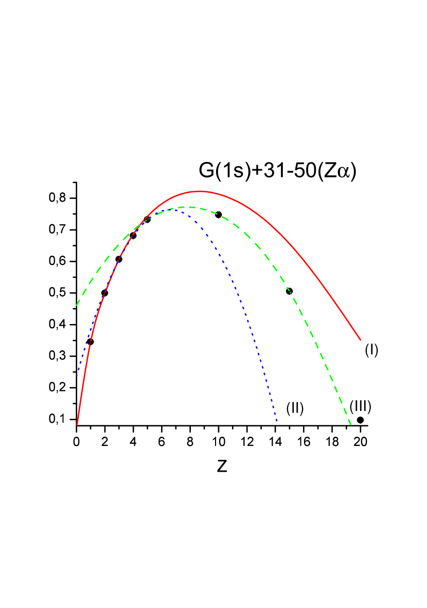
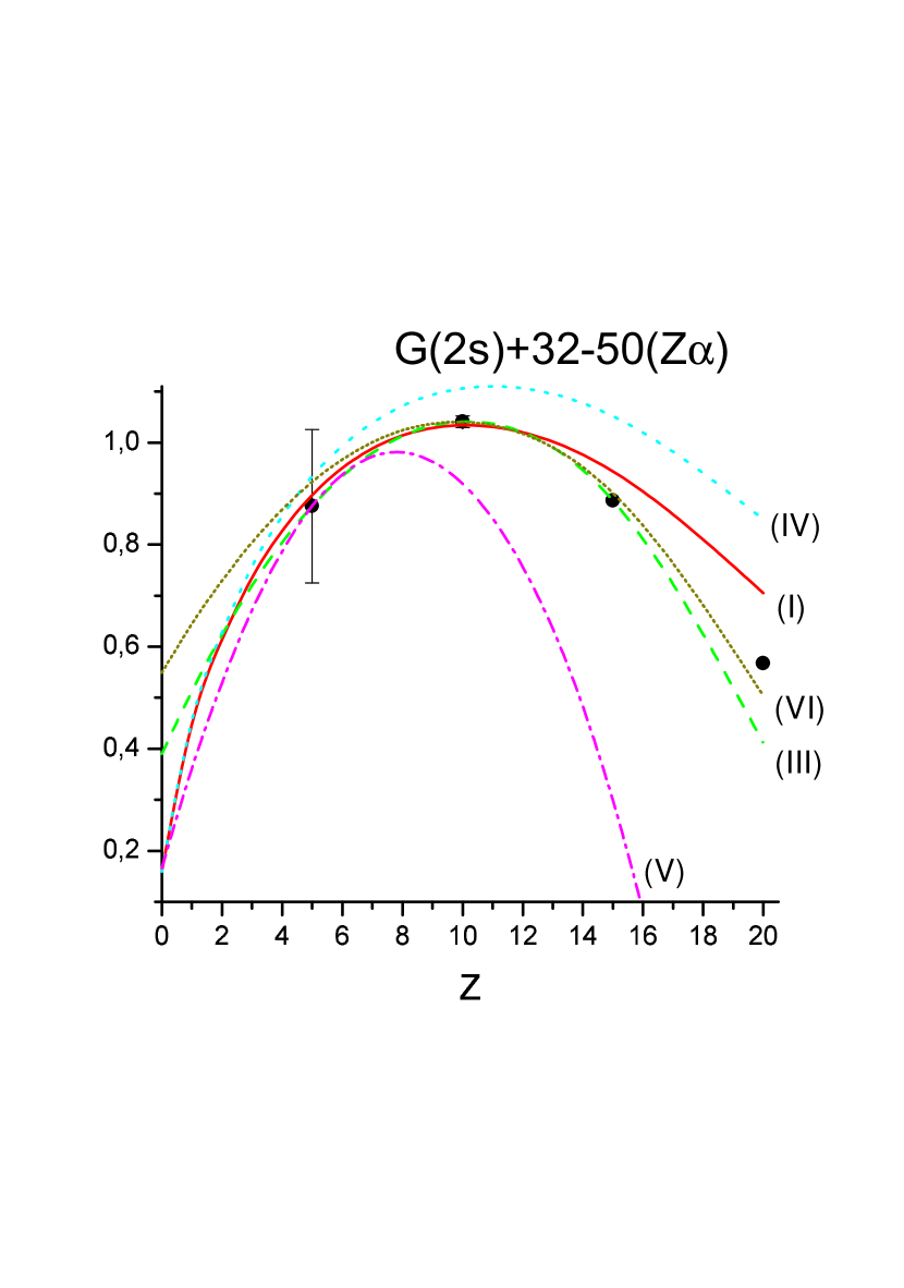
Figure 1: Fitting of $G(Z)$ for 1s and 2s states.

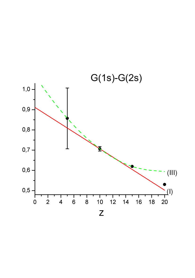
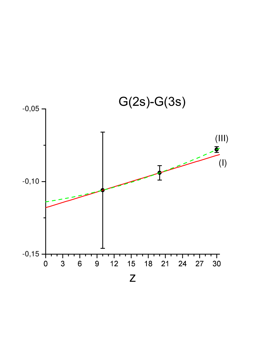
Figure 2: Fitting of $G_{1s}(Z)-G_{2s}(Z)$ and $G_{2s}(Z)-G_{3s}(Z)$.

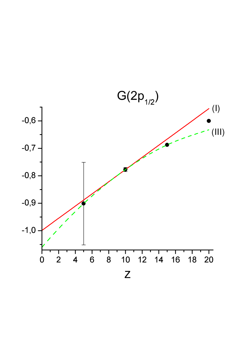
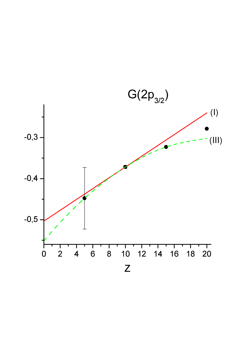
Figure 3: Fitting of $G(Z)$ for the 2p_1/2 and 2p_3/2 states.

The results of all fits for $Z=2$ are summarized in Table 2 and $Z=7$ in Table 3. The value for the $1s$ state at $Z=7$ is in agreement with the less accurate one obtained in Ref. yer .

Table 2: Values $G(2)$ for different types of fitting

Value	(I)	(IV)
$G_{1s}$	-29.772(7)
$G_{2s}$	-30.7(2)	-30.64(3)
$G_{1s}-G_{2s}$	0.87(3)
$G_{2s}-G_{3s}$	-0.12(9)
$G_{2p_{1/2}}$	-0.95(3)
$G_{2p_{3/2}}$	-0.48(3)

Table 3: Values $G(7)$ for different types of fitting

Value	(I)	(II)	(III)	(IV)	(V)	(VI)
$G_{1s}$	-27.6(1)	-27.68(1)	-27.677(9)
$G_{2s}$	-28.5(1)		-28.47(5)	-28.4(1)	-28.47(5)	-28.45(3)
$G_{1s}-G_{2s}$	0.77(3)		0.79(5)
$G_{2p1/2}$	-0.84(3)		-0.85(5)
$G_{2p3/2}$	-0.41(3)		-0.41(3)

2.6 Two-loop contributions

Two-loop corrections have not yet been calculated exactly and only a few of the terms have been known up-to-date two5 ; jetp93 :

$$H_{ns}(Z)= \left(-\frac{2179}{648}-\frac{10}{27}\pi^{2}+\frac{3}{2}\pi^{2}\ln(2)-\frac{9}{4}\zeta(3)\right)-21.556(3)\,(Z\alpha)$$ (25)

$$+ (Z\alpha)^{2}\left[-\frac{8}{27}\,\ln^{3}\frac{1}{(Z\alpha)^{2}}+G^{II}_{ns}(Z)\right]\,,$$

$$H_{2p_{1/2}}(Z)= - \frac{1}{3}\,a_{4}+(Z\alpha)^{2}\left[\frac{1}{9}\,\ln^{2}\frac{1}{(Z\alpha)^{2}}+G^{II}_{2p_{1/2}}(Z)\right]\,,$$ (26)

$$H_{2p_{3/2}}(Z)= \frac{1}{6}\,a_{4}+(Z\alpha)^{2}\left[\frac{1}{9}\,\ln^{2}\frac{1}{(Z\alpha)^{2}}+G^{II}_{2p_{1/2}}(Z)\right]\,,$$ (27)

where for $l\neq 0$ the leading contribution is due to the anomalous magnetic moment of the electron

$$a_{4}=\frac{197}{144}+\frac{\pi^{2}}{12}-\frac{\pi^{2}}{2}\ln(2)+\frac{3}{4}\zeta(3)\simeq-0.328\,478\,966\dots\,.$$ (28)

The higher-order terms denoted as $G^{II}(Z)$ are not known. We expect karshenboim99 that the magnitude of $G^{II}$ does not exceeded by half the value of the leading logarithmic term ($\ln^{3}(Z\alpha)$ for the $ns$ states and $\ln^{2}(Z\alpha)$ for the $2p$ states) at $Z=1$ and use the estimation for $G^{II}(1)$ for any $Z$. The purpose of this calculation is to eliminate any other sources of theoretical uncertainty and to study a value of $G^{II}_{2s}$ by a comparison with experiment.

The leading state-dependent term for the $s$-state is also known jpb ; zp97 , and in particular one can find

$$H_{1s}(Z)-H_{2s}(Z) = (Z\alpha)^{2}\left[\ln^{2}\frac{1}{(Z\alpha)^{2}}\left(\frac{16}{9}\ln(2)-\frac{7}{3}\right)+G^{II}_{12}(Z)\right]\,,$$ (29)

$$H_{2s}(Z)-H_{3s}(Z) = (Z\alpha)^{2}\left[\ln^{2}\frac{1}{(Z\alpha)^{2}}\left(\frac{16}{9}\ln\frac{3}{2}-\frac{91}{81}\right)+G^{II}_{23}(Z)\right]\,,$$ (30)

and unknown higher-order contributions $G^{II}$ are estimated in the same way as for the $2p$ states.

2.7 Three-loop contributions

The three-loop contributions for $ns$ state at $Z=0$ was eventually obtained in Ref. meln

$$K_{ns}(0)=0.4174\dots\,,$$ (31)

while for the $p$-states the corrections

$$K_{2p_{1/2}}(0) = -\frac{1}{3}\,a_{6}\,,$$ (32)

$$K_{2p_{3/2}}(0) = \frac{1}{6}\,a_{6}\,,$$ (33)

comes from the $g\!-\!2$ of electron:

$$a_{6}=1.181\,241\dots$$ (34)

2.8 Pure recoil corrections

The pure recoil correction

$$\Delta E_{\rm Rec}=\frac{1}{\pi}\,\frac{1}{n^{3}}\,\frac{m^{2}}{M}(Z\alpha)^{4}R(Z)\;,$$ (35)

where is known analytically with sufficient accuracy recoil

$$R_{ns}(Z)= (Z\alpha)\left[\frac{2}{3}\ln\frac{1}{(Z\alpha)}-\frac{8}{3}\ln\big{(}k_{0}(ns)\big{)}+\frac{187}{18}\right]$$ (36)

$$+ (Z\alpha)^{2}\,\pi\left(4\ln(2)-\frac{7}{2}\right)\,,$$

$$R_{2p}(Z)= (Z\alpha)\,\left[-\frac{8}{3}\ln\big{(}k_{0}(2p)\big{)}-\frac{7}{18}\right]+(Z\alpha)^{2}\,\frac{\pi}{3}\;.$$ (37)

Some numerical results for the states with $n=1,2$ are also available numrec . Second-order recoil corrections ($(Z\alpha)^{4}(m^{3}/M^{2})$) are known recoil2 but their contribution is negligible.

2.9 Radiative-recoil corrections

The radiative-recoil corrections are known only in the leading order pach952

$$\Delta E_{\rm RRC}(nl)=\frac{\alpha(Z\alpha)^{5}}{\pi}\,\frac{m}{n^{3}}\,\frac{m}{M}\,\left(-1.36449\right)\,\delta_{l0}\,.$$ (38)

2.10 Finite-nuclear-size correction

The correction for $s$-states due to the finite size of the nucleus is of the form

$$\Delta E_{\rm Nucl}(nl)=\frac{2}{3}\frac{(Z\alpha)^{4}\,m}{n^{3}}\,\Big{(}m\,R_{\rm N}\Big{)}^{2}\,\delta_{l0}\,\left(1+(Z\alpha)^{2}\ln\frac{1}{Z\alpha m\,R_{\rm N}}\right)\,,$$ (39)

where $R_{N}$ is the rms nuclear charge distribution radius. The leading term in Eq. (39) vanishes for the $p$ states because their non-relativistic wave function is vanishes at the origin itself. However, the small component of the Dirac wave function contains a factor of ${\bf\sigma}{\bf p}/2m$ and the Dirac wave function is not equal to zero at the origin. In particular, one can easily find

$$\Bigl{(}\Psi_{2p_{1/2}}(0)\Bigr{)}^{2} = {3\over 32}\frac{(Z\alpha)^{5}m^{3}}{\pi}\;,$$

$$\Bigl{(}\Psi_{2p_{3/2}}(0)\Bigr{)}^{2} = 0\;,$$ (40)

and

$$\Delta E_{\rm Nucl}(2p_{1/2}) = {1\over 16}\,(Z\alpha)^{6}\,m\,\Big{(}m\,R_{\rm N}\Big{)}^{2}\,\;,$$

$$\Delta E_{\rm Nucl}(2p_{3/2}) = 0\;.$$ (41)

The error of the logarithmic term can be estimated as $1/2\,\Delta E_{\rm Nucl}\,(Z\alpha)^{2}\ln(1/\alpha)$. The nuclear radii and corrections are presented in Table 4.

Table 4: Nuclear square charge radius

Atom	$R_{\rm N}$	$\Delta E_{\rm Nucl}(2s)$	Ref.
	[fm]	[MHz]
${}^{4}{\rm He}$	1.674(12)	8.80(12)	RHe4
${}^{14}{\rm N}$	2.560(11)	3145(33)	RN14
${}^{15}{\rm N}$	2.612(9)	3274(30)	RN15

3 Summary

All contributions and final values of the Lamb shifts in the lowest states of hydrog-like ions ⁴He⁺, ¹⁴N⁶⁺ and ¹⁵N⁶⁺ are presented in Tables 5, 6 and 7, respectively. The final results for intervals which can be measured are listed in Table 8. The results in Table 8 involve three main sources of uncertainty and we split the uncertainty there and in auxiliary Tables 5–7, respectively:

• The higher-order two-loop corrections;

• Nuclear structure corrections (They require further study);

• Other theoretical QED uncertainties beyond the higher-oder two-loop effects.

The theory (with unknown higher-order two-loop effects excluded) is found to be accurate enough and we hope the study of helium and nitrogen hydrogen-like ions is a promising way to study in detail the two-loop contributions experimentally.

Table 5: Different contributions to the Lamb shift in hydrogen-like helium ${}^{4}{\rm He}$ (in MHz)

Contribution	$2s$		$2p_{1/2}$		$2p_{3/2}$
SE	14 251	.51(2)	-204	.747(10)	201	.503(10)
VP	-426	.78	-0	.022	-0	.005
WK	0	.02	0		0
One-loop	13 824	.75(2)	-204	.769(10)	201	.498(10)
Two-loop	0	.70(11)	0	.420(2)	-0	.201(2)
Three-loop	0	.004	0	.003	0	.002
Pure recoil	2	.53	-0	.131	-0	.131
Radiative recoil	-0	.01	0		0
QED	13 827	.98(11)(2)	-204	.484(2)(10)	201	.168(2)(10)
Nuclear size	8	.80(13)	0		0
Total	13 836	.77(11)(13)(2)	-204	.484(2)(10)	201	.168(2)(10)

Table 6: Different contributions to the Lamb shift in ¹⁴N (in MHz)

Contribution	$2s$		$2p_{1/2}$		$2p_{3/2}$
SE	1 390 601	(19)	-29 298	(19)	31 088	(19)
VP	-62 021		-40		-8
WK	32		0		0
One-loop	1 328 611	(19)	-29 338		31 080
Two-loop	-411	(209)	68	(2)	-25	(2)
Three-loop	0	.5	-0	.5	0	.3
Pure recoil	319		-17		-17
Radiative recoil	-2		0		0
QED	1 328 517	(209)(19)	-29 287	(2)(19)	31 038	(2)(19)
Nuclear size	3 145	(33)	6		0
Total	1 331 662	(209)(33)(19)	-29 282	(2)(19)	31 038	(2)(19)

Table 7: Different contributions to the Lamb shift in ¹⁵N (in MHz)

Contribution	$2s$		$2p_{1/2}$		$2p_{3/2}$
SE	1 390 611	(19)	-29 298	(19)	31 088	(19)
VP	-62 022		-40		-8
WK	32		0		0
One-loop	1 328 620	(19)	-29 338		31 080
Two-loop	-411	(209)	68	(2)	-25	(2)
Three-loop	0	.5	-0	.5	0	.3
Pure recoil	297		-16		-16
Radiative recoil	-2		0		0
QED	1 328 505	(209)(19)	-29 286	(2)(19)	31 039	(2)(19)
Nuclear size	3 274	(30)	6		0
Total	1 331 779	(209)(30)(19)	-29 280	(2)(19)	31 039	(2)(19)

Table 8: Differences of energies (in MHz)

Atom	Value	Result
${}^{4}{\rm He}$	$\Delta E(2s-2p_{1/2})$	14 041.25(11)(13)(2)
${}^{4}{\rm He}$	$8E_{L}(2s)-27E_{L}(3s)$	-768.35(29)
${}^{14}{\rm N}$	$\Delta E(2p_{3/2}-2s)$	25 030 522(209)(33)(27)
${}^{15}{\rm N}$	$\Delta E(2p_{3/2}-2s)$	25 030 475(209)(30)(27)

References

- (1) S. G. Karshenboim, invited talk at ICAP 2000, to be published, e-print hep-ph/0007278
- (2) S. G. Karshenboim, invited talk at MPLP 2000, to be published, e-print physics/0008215
- (3) S. G. Karshenboim, Can. J. Phys. 77, 241 (1998)
- (4) R. Pohl et al., this conference
- (5) T. W. Hänsch, this conference
- (6) C. Schwob et al., this conference
- (7) G. W. F. Drake and A. van Wijngaarden, this conference
- (8) S. A. Burrows et al., this conference
- (9) E. G. Myers and M. R. Tarbutt, this conference
- (10) S. Mallampalli and J. Sapirstein, Phys. Rev. Lett. 80, 5297 (1998)
- (11) I. Goidenko et al., Phys. Rev. Lett. 83, 2312 (1999); this conference
- (12) V. A. Yerokhin, this conference
- (13) S. G. Karshenboim, Z. Phys. D 39, 109 (1997)
-
(14)
S. Klarsfeld and A. Maquet, Phys. Lett. B43, 201 (1973);
G. W. F. Drake and R. A. Swainson, Phys. Rev. A41, 1243 (1990) - (15) S. G. Karshenboim, Can. J. Phys. 76, 168 (1998); JETP 89, 1575 (1999)
- (16) V. G. Ivanov and S. G. Karshenboim. Phys. At. Nucl. 60, 270 (1997)
- (17) N. L. Manakov, A. A. Nekipelov and A. G. Fainshtein, JETP 68, 673 (1989)
- (18) W. R. Johnson and G. Soff, At. Data. Nucl. Data Tables 33, 405 (1985)
- (19) K. Pachucki, Ann. Phys. (N. Y.) 226, 1 (1993)
- (20) U. D. Jentschura and K. Pachucki, Phys. Rev. A82, 1853 (1996)
- (21) P. J. Mohr, Phys. Rev. A46, 4421 (1992)
- (22) U. D. Jentschura et al., Phys. Rev. Lett. 82, 53 (1999)
- (23) S. G. Karshenboim, JETP 79, 230 (1994)
- (24) P. J. Mohr and Y.-K. Kim, Phys. Rev. A45, 2727 (1992)
- (25) V. A. Yerokhin, private communication
-
(26)
K. Pachucki and H. Grotch, Phys. Rev. A 51, 1854 (1995);
E. A. Golosov, A. S. Elkhovski, A. I. Mil’shten, and I. B. Khriplovich, JETP 80, 208 (1995) - (27) A. N. Artemyev, V. M. Shabaev, and V. A. Yerokhin, Phys. Rev. A 52, 1884 (1995); J. Phys. B 28, 5201 (1995)
-
(28)
W. A. Barker and F. N. Glover, Phys. Rev. 99, 317 (1955);
S. J. Brodsky and R. G. Parsons, Phys. Rev. 163, 134 (1967); 176, 423E (1968);
K. Pachucki and S. G. Karshenboim, J. Phys. B 28, L221 (1995) - (29) K. Pachucki, Phys. Rev. A52, 1079 (1995)
-
(30)
K. Pachucki, Phys. Rev. Lett. 72, 3154 (1994);
M. I. Eides and V. A. Shelyuto, Phys. Rev. A52, 954 (1995) - (31) S. G. Karshenboim, JETP 76, 541 (1993)
- (32) T Kinoshita, this conference
- (33) S. G. Karshenboim, JETP 82, 403 (1996); J. Phys. B29, L21 (1996)
- (34) K. Melnikov and T. van Ritbergen, this conference
- (35) I. Sick, J. S. McCarthy and R. R. Whitney, Plys. Lett. B 64, 33 (1976)
- (36) L. A. Schaller, L. Schellenberg, A. Rusetschi and H. Schneuwly, Nucl. Phys. A343, 333 (1980)
- (37) J. W. de Vries, D. Doornhof, C. W. de Jager, R. P. Singhal, S. Salem, G. A. Peterson and R. S. Hicks, Phys. Lett. B205, 22 (1988)