Study Notes on Numerical Solutions of the Wave Equation with the Finite Difference Method

Preface

The simulation of the dynamics of classical field theories is currently gaining some attention from the high-energy community, mainly in the context of statistical field theory. Recent papers show that, in some particular but important conditions, classical field theories are a very good approximation to the quantum evolution of fields at finite temperature (see, for instance, [1, 2]). Also, in the context of condensed-matter systems, the dynamics of effective classical fields has proven to be a very efficient tool in describing both the equilibrium and non-equilibrium properties of systems such as ferromagnets [3]. In order to simulate these theories, they must be first discretized and cast on a lattice, a job far from trivial to do in a consistent manner [4]. After the discretization, the differential equations of motion transform themselves into finite difference equations. Before doing any sort of useful calculation in the physical context above, one is supposed to understand the basic foundations of the numerical method, the study of which is the objective of this monograph.

Following this motivation, I will present, in an introductory way, the Finite Difference method for hyperbolic equations, focusing on a method which has second order precision both in time and space (the so-called staggered leapfrog method) and applying it to the case of the 1d and 2d wave equation. A brief derivation of the energy and equation of motion of a wave is done before the numerical part in order to make the transition from the continuum to the lattice clearer.

To illustrate the extension of the method to more complex equations, I also add dissipative terms of the kind $-\eta\dot{u}$ into the equations. I also briefly discuss the von Neumann numerical stability analysis and the Courant criterion, two of the most popular in the literature. In the end I present some numerical results obtained with the leapfrog algorithm, illustrating the importance of the lattice resolution through energy plots.

I have tried to collect, in a concise way, the main steps necessary to have a stable algorithm to solve wave-like equations. More sophisticated versions of these equations should be handled with care, and accompanied of a rigorous study of convergence and stability which could be found in the references cited in the end of this work.

Contents

1. 1 The Wave Equation
   1. 1.1 Introduction
   2. 1.2 Waves in 1-dimension (the free string)
      1. 1.2.1 Equation of Motion
      2. 1.2.2 Energy
   3. 1.3 Waves in 2-dimensions (the free membrane)
      1. 1.3.1 Equation of Motion
      2. 1.3.2 Energy
2. 2 Finite Differences
   1. 2.1 Introduction
   2. 2.2 Difference Equations
   3. 2.3 The von Neumann Stability Analysis
   4. 2.4 The Courant Condition
   5. 2.5 The Staggered Leapfrog Algorithm
3. 3 Examples
   1. 3.1 The Free String (1D)
   2. 3.2 The Membrane (2D)
4. A Taylor’s Theorem
   1. A.1 Definitions
   2. A.2 Useful Expansions

Chapter 1 The Wave Equation

1.1 Introduction

Partial Differential Equations (from now on simply PDEs) are divided in the literature basically in three kinds: parabolic, elliptic and hyperbolic (the criterion of classification of these equations can be found in [5, Chap. 8]). In this work we will be interested mainly on hyperbolic equations, of which the wave equation is the paradigm:

$$\nabla^{2}u=\frac{1}{v^{2}}\frac{\partial^{2}u}{\partial t^{2}},$$ (1.1)

where $v^{2}=\frac{\tau}{\lambda}$ is the square of the wave velocity in the medium, which in the case of a free string could be determined by the tension $\tau$ and the mass density per length unit $\lambda$.

From the strict numerical point of view, the distinction between these classes of PDEs isn’t of much importance [6]. There is, however, another sort of classification of PDEs which is relevant for numerical purposes: the initial value problems (which include the case of the hyperbolic equations) and the boundary condition problems (which include, for instance, parabolic equations). In this work we will restrict ourselves to initial value problems. See reference [6] for a good introduction to boundary condition problems.

In the equation (1.1) we could still add a dissipative term proportional to the first power of the time derivative of $u$, i.e.,

$$\tau\nabla^{2}u=\lambda\frac{\partial^{2}u}{\partial t^{2}}+\eta\frac{\partial u}{\partial t},$$ (1.2)

where $\eta$ is the viscosity coefficient.

Our first step will be to derive the wave equation from a simple mechanical analysis of the free rope. Being this a well known problem in classical mechanics, we will go through only the main steps of it (for a more complete treatment of the problem of the free string, see, for example, [7, Chaps. 8 and 9]). Once we are done with the 1-d wave equation, we will proceed further to the 2-d case, which isn’t as abundant in the literature as the 1-d case.

1.2 Waves in 1-dimension (the free string)

1.2.1 Equation of Motion

Figure 1.1: Representing the tension forces acting on an infinitesimal element of the rope.

Figure 1.1 gives us an idea of a mass element $dm$ with linear dimension $dx$ subject to tension forces. We are interested on the vertical displacement of this mass element, so, for this direction, we could write the resulting force:

$$dF_{u}=\left.\vec{\tau}\cdot\hat{u}\right|_{x+dx}-\left.\vec{\tau}\cdot\hat{u}\right|_{x},$$ (1.3)

where $\vec{\tau}$ is the tension and the unit vector $\hat{u}$ refers to the vertical direction. Within the domain of smooth deformations of the string (i.e., small $\beta$), we could write:

$$\tau_{u}\equiv\vec{\tau}\cdot\hat{u}=\tau\sin\beta\approx\tau\tan\beta=\tau\frac{\partial u}{\partial x}$$ (1.4)

We notice now that (1.3) could be written as:

$$dF_{u}=\frac{\left.\tau_{u}\right|_{x+dx}-\left.\tau_{u}\right|_{x}}{dx}dx=\frac{\partial\tau_{u}}{\partial x}dx=\frac{\partial}{\partial x}\left(\tau\frac{\partial u}{\partial x}\right)dx$$

We will now restrict ourselves to the case of constant tensions along the rope, so that:

$$dF_{u}=\tau\frac{\partial^{2}u}{\partial x^{2}}dx$$ (1.5)

Equating this with Newton’s second law

$$dF_{u}=dm\frac{\partial^{2}u}{\partial t^{2}}=\lambda\frac{\partial^{2}u}{\partial t^{2}}dx,$$

where $\lambda$ is the linear mass density, we obtain then the wave equation for a free string:

$$\tau\frac{\partial^{2}u}{\partial x^{2}}=\lambda\frac{\partial^{2}u}{\partial t^{2}}$$ (1.6)

1.2.2 Energy

The kinetic energy could be evaluated in a straightforward manner, integrating the kinetic energy term for a representative mass element:

$$dT=\frac{1}{2}dm\cdot v_{u}^{2},$$

with $dm=\lambda\cdot dx$ and $v_{u}=\frac{\partial u}{\partial t}$, in other words,

$$T=\int dT=\frac{\lambda}{2}\int_{0}^{l}\left(\frac{\partial u}{\partial t}\right)^{2}dx$$ (1.7)

The potential energy can be obtained by calculating the work necessary to bring the string from a “trivial” configuration $u(x,0)=0$ to the configuration at which we want to evaluate the potential energy $u(x,t)$. We will fix the boundary conditions $u(0,t)=u(l,t)=0$ (string tied at the ends) and as a consequence of this, $\partial_{t}u(0,t)=\partial_{t}u(l,t)=0$. The potential energy relative to the work necessary to change of $\delta u$ the configuration of an element of the string in an interval of time $dt$ is:

$$\delta V=-dF_{u}\cdot\delta u=-dF_{u}\cdot\left(\frac{\partial u}{\partial t}\right)dt$$

Therefore, the potential energy of the whole string in this same interval of time is:

$$dV=-dt\cdot\int dF_{u}\left(\frac{\partial u}{\partial t}\right)$$

Substituting (1.5) in the latter we get:

$$dV=-dt\cdot\int_{0}^{l}\tau\left(\frac{\partial^{2}u}{\partial x^{2}}\right)\left(\frac{\partial u}{\partial t}\right)dx$$

We are however interested on $V\left[u(x,t)\right]$, so integrating in time and using the boundary conditions above, we have:

$$V = \int dV=-\tau\int_{0}^{t}dt\int_{0}^{l}dx\left(\frac{\partial u}{\partial t}\right)\left(\frac{\partial^{2}u}{\partial x^{2}}\right)=$$

$$= -\tau\int_{0}^{t}dt\left\{\left.\frac{\partial u}{\partial t}\frac{\partial u}{\partial x}\right|_{0}^{l}-\int_{0}^{l}\frac{\partial u}{\partial x}\frac{\partial^{2}u}{\partial x\partial t}dx\right\}=$$

$$= \tau\int_{0}^{t}dt\int_{0}^{l}\frac{\partial u}{\partial x}\frac{\partial^{2}u}{\partial x\partial t}dx=$$

$$= \tau\int_{0}^{t}dt\frac{1}{2}\frac{\partial}{\partial t}\int_{0}^{l}\left(\frac{\partial u}{\partial x}\right)^{2}dx=$$

$$= \frac{\tau}{2}\left.\int_{0}^{l}\left(\frac{\partial u}{\partial x}\right)^{2}dx\right|_{0}^{t}\Rightarrow$$

$$V=\frac{\tau}{2}\int_{0}^{l}\left(\frac{\partial u}{\partial x}\right)^{2}dx$$ (1.8)

With (1.7) and (1.8) we have finally the total energy of the rope:

$$E=\frac{\lambda}{2}\int_{0}^{l}\left(\frac{\partial u}{\partial t}\right)^{2}dx+\frac{\tau}{2}\int_{0}^{l}\left(\frac{\partial u}{\partial x}\right)^{2}dx$$ (1.9)

In our applications we will take $\lambda=\tau$ such that $v^{2}=1$ and (1.9) assumes the simple form:

$$E=\frac{1}{2}\int_{0}^{l}\left[\left(\frac{\partial u}{\partial t}\right)^{2}+\left(\frac{\partial u}{\partial x}\right)^{2}\right]dx$$ (1.10)

This energy equation will be very useful to test our algorithms through an analysis of conservation (or dissipation) during the dynamical evolution of the system.

1.3 Waves in 2-dimensions (the free membrane)

1.3.1 Equation of Motion

Figure 1.2: Representing a mass element $dm$ of dimensions $dxdy$. The element is subject to tension forces on each side (analogous to the borders of the mass element in the 1-d case), being these forces orthogonal to the axes of the sides. Only the variation with respect to $x$ of $u$ is drawn (i.e., $u$ and $u+du$ in the figure are displacements of $u(x,y)$ keeping $y$ constant and varying $x$).

In its two dimensional version, the wave equation could be describing a membrane, a liquid surface, or some “coarse-grained” field in the surface physics, to cite a few. In the case of the membrane or other elastic surface, the oscillations are also constrained to be small (analogously to the 1-d string).

We notice now that the additional dimension forces us to define the tension “per unit length”:

$$f=\frac{\tau}{l}$$ (1.11)

This force per unit length could be understood with a simple example: stretch a tape of width $l$ from its extremities with force $\tau$. We can’t ask the force on a point of the tape, but only on some element of some definite length and width (of course, this element could be differential, playing the same role of a linear differential element in the case of the string). Formula (1.11), times the length of the element, then gives you the resulting force (tension) on the element. In this way, we extend the equation (1.3) to two dimensions:

$$dF_{u}=\left[\left.\vec{f}_{x}\cdot\hat{u}\right|_{x+dx,y}dy-\left.\vec{f}_{x}\cdot\hat{u}\right|_{x,y}dy\right]+\left[\left.\vec{f}_{y}\cdot\hat{u}\right|_{x,y+dy}dx-\left.\vec{f}_{y}\cdot\hat{u}\right|_{x,y}dx\right],$$ (1.12)

where $\left.\vec{f}_{x}\cdot\hat{u}\right|_{x,y}dy\equiv\left.f_{x,u}\right|_{x,y}dy$ is the $x$ component of the tension in the direction $\hat{u}$ acting on the side defined by the points $(x,y)$ e $(x,y+dy)$, and so on. We are going to suppose that the forces on the sides of the elements are orthogonal to their axes, which is the same as decomposing the tension force on $dm$ into four components, one for each side (notice, however, that we have effectively only two resulting components, to wit $\hat{x}$ and $\hat{y}$). Doing this we won’t need to emphasize the tension components along $x$ or $y$, $\left.\vec{f}_{x}\cdot\hat{u}\right|_{x,y}$ becoming simply $\left.f_{u}\right|_{x,y}$ and so on. Nevertheless it is still important, for what we said above, to know what side we are talking about. So, in the regime of small vibrations (i.e., small angles of deformation), we could find $f_{u}$ analogously to the string case

$$f_{u}dy = f\frac{\partial u}{\partial x}dy$$ (1.13)

$$f_{u}dx = f\frac{\partial u}{\partial y}dx,$$ (1.14)

where $f_{u}dy$ and $f_{u}dx$ are the tensions in the direction $\hat{u}$ on a side of length $dy$ and $dx$ along $y$ and $x$, respectively. We emphasize that, with this notation plus the knowledge of the point where we are going to evaluate the derivatives, we have a complete specification of the side on which the tension acts. With all this in hands, Eq. (1.12) becomes:

$$dF_{u}=\left[\left.f_{u}\right|_{x+dx,y}dy-\left.f_{u}\right|_{x,y}dy\right]+\left[\left.f_{u}\right|_{x,y+dy}dx-\left.f_{u}\right|_{x,y}dx\right]$$

With calculations analogous to those of the previous section, we have:

$$dF_{u} = \frac{\left.f_{u}\right|_{x+dx,y}-\left.f_{u}\right|_{x,y}}{dx}dxdy+\frac{\left.f_{u}\right|_{x,y+dy}-\left.f_{u}\right|_{x,y}}{dy}dydx=$$ (1.15)

$$= \frac{\partial f_{u}}{\partial x}dxdy+\frac{\partial f_{u}}{\partial y}dxdy=$$ (1.16)

$$= f\frac{\partial^{2}u}{\partial x^{2}}dxdy+f\frac{\partial^{2}u}{\partial y^{2}}dxdy$$ (1.17)

With Newton’s second law we obtain:

$$f\frac{\partial^{2}u}{\partial x^{2}}dxdy+f\frac{\partial^{2}u}{\partial y^{2}}dxdy = dm\frac{\partial^{2}u}{\partial t^{2}}\Rightarrow$$

$$f\frac{\partial^{2}u}{\partial x^{2}}dxdy+f\frac{\partial^{2}u}{\partial y^{2}}dxdy = \sigma dxdy\frac{\partial^{2}u}{\partial t^{2}}\Rightarrow$$

$$f\left(\frac{\partial^{2}u}{\partial x^{2}}+\frac{\partial^{2}u}{\partial y^{2}}\right) = \sigma\frac{\partial^{2}u}{\partial t^{2}}\Rightarrow$$

$$\frac{\partial^{2}u}{\partial x^{2}}+\frac{\partial^{2}u}{\partial y^{2}}=\frac{1}{v^{2}}\frac{\partial^{2}u}{\partial t^{2}},$$ (1.18)

which is the desired wave equation for two dimensions, with $v^{2}=\frac{f}{\sigma}$ and $\sigma$ the surface mass density.

1.3.2 Energy

The derivation of the total energy is done in the same manner as the 1d case. We will consider a surface $z=u(x,y,t)$ with support of dimension $l\times l$, subject to the boundary conditions $\left.u\right|_{boundary}\equiv u(0,y,t)=u(l,y,t)=u(x,0,t)=u(x,l,t)=0$ and $\left.\dot{u}\right|_{boundary}\equiv\dot{u}(0,y,t)=\dot{u}(l,y,t)=\dot{u}(x,0,t)=\dot{u}(x,l,t)=0$, where $\dot{u}\equiv\partial u/\partial t$. Let us begin with the kinetic term:

$$dT = \frac{1}{2}dm\cdot\dot{u}^{2}=\frac{\sigma}{2}\dot{u}^{2}dxdy\Rightarrow$$ (1.19)

$$T = \frac{\sigma}{2}\int_{0}^{l}\int_{0}^{l}\left(\frac{\partial u}{\partial t}\right)^{2}dxdy,$$ (1.20)

where $\sigma$ is the surface mass density.

The potential energy is obtained in an analogous way to the Section (1.2):

$$dV = -dt\cdot\int dF_{u}\left(\frac{\partial u}{\partial t}\right)=$$

$$= -dt\cdot\int_{0}^{l}\int_{0}^{l}f\left(\frac{\partial^{2}u}{\partial x^{2}}+\frac{\partial^{2}u}{\partial y^{2}}\right)\left(\frac{\partial u}{\partial t}\right)dxdy\Rightarrow$$

$$V = -f\int_{0}^{t}dt\left\{\int_{0}^{l}dy\int_{0}^{l}dx\left(\frac{\partial^{2}u}{\partial x^{2}}\frac{\partial u}{\partial t}\right)+\int_{0}^{l}dx\int_{0}^{l}dy\left(\frac{\partial^{2}u}{\partial y^{2}}\frac{\partial u}{\partial t}\right)\right\}=$$

$$= f\int_{0}^{t}dt\left\{\int_{0}^{l}dy\frac{1}{2}\frac{\partial}{\partial t}\int_{0}^{l}\left(\frac{\partial u}{\partial x}\right)^{2}dx+\int_{0}^{l}dx\frac{1}{2}\frac{\partial}{\partial t}\int_{0}^{l}\left(\frac{\partial u}{\partial y}\right)^{2}dy\right\}=$$

$$= \frac{f}{2}\int_{0}^{t}dt\frac{\partial}{\partial t}\left\{\int_{0}^{l}\int_{0}^{l}\left[\left(\frac{\partial u}{\partial x}\right)^{2}+\left(\frac{\partial u}{\partial y}\right)^{2}\right]dxdy\right\}=$$

$$= \frac{f}{2}\left.\int_{0}^{l}\int_{0}^{l}\left[\left(\frac{\partial u}{\partial x}\right)^{2}+\left(\frac{\partial u}{\partial y}\right)^{2}\right]dxdy\right|_{0}^{t}\Rightarrow$$

$$V=\frac{f}{2}\int_{0}^{l}\int_{0}^{l}\left[\left(\frac{\partial u}{\partial x}\right)^{2}+\left(\frac{\partial u}{\partial y}\right)^{2}\right]dxdy$$ (1.21)

Then the total energy for our usual condition $f=\sigma\Rightarrow v^{2}=1$ is:

$$E=\frac{1}{2}\int_{0}^{l}\int_{0}^{l}\left[\left(\frac{\partial u}{\partial x}\right)^{2}+\left(\frac{\partial u}{\partial y}\right)^{2}+\left(\frac{\partial u}{\partial t}\right)^{2}\right]dxdy$$

or, in a more general way (we are going to take as granted the result for more than two dimensions),

$$E=\int d^{n}\vec{r}\left[\frac{1}{2}(\vec{\nabla}u)^{2}+\frac{1}{2}\dot{u}^{2}\right]$$

Once again I emphasize that these results are important for the verification of the stability of our numerical analysis. This derivation is shown here not only as an exercise, but also because I couldn’t find the 2-d version in any textbook.

Chapter 2 Finite Differences

2.1 Introduction

Differently from the non-approximate analytical solutions of PDEs in the continuum (for instance, those obtained through variable separation and subsequent integration), numerical solutions obtained in a computer have limited precision. It is due to the way in which computers store data and also because of their limited memory. After all, how could we write in decimal notation (or in any other base) an irrational number like $\sqrt{2}$ making use of a finite number of digits? In this work we won’t stick with rigorous derivations of the theorems nor of most of the results presented. The references listed in the end should be considered for this end.

The central idea of numerical methods is quite simple: to give finite precision (“the discrete”) to those objects endowed with infinite precision (“the continuum”). By discretize we understand to transform continuum variables like $x,y,..,z$ into a set of discrete values $\{x_{i}\},\{y_{i}\},...,\{z_{i}\}$, where $i$ runs over a finite number of values, thus sampling the wholeness of the original variables. As a consequence of this discretization, integrals become sums and derivatives turns out to mere differences of finite quantities (hence the name “finite differences”). I illustrate below these ideas:

$$\int f(x)dx = \lim_{\delta x\rightarrow 0}\sum_{n}f(n\delta x)\delta x\,\rightarrow\,\sum_{n}f(n\Delta x)\Delta x$$ (2.1)

$$\frac{df(x)}{dx} = \lim_{\delta x\rightarrow 0}\frac{f(x+\delta x)-f(x)}{\delta x}\,\rightarrow\,\frac{f(x+\Delta x)-f(x)}{\Delta x},$$ (2.2)

where $\delta x$ is a variable with infinite precision (thus its value could be as small as we want) and $\Delta x\ll 1$ is a variable with finite precision, which under the computational point of view is the limiting case analogous to $\delta x$. We could naively expect that, the smaller the value of $\Delta x$, the closer we are to the continuum theory. This would be indeed true if computers didn’t have finite precision! The closer your significant digits get to the limiting precision of the computer, the worse is your approximation, because it will introduce the well-known “round-off errors”, which are basically truncation errors. The reference [8] has a somewhat lengthy discussion about computational issues like this.

2.2 Difference Equations

Difference equations are to a computer in the same way as differential equations are to a good mathematician. That is, if you have a problem in the form of a differential equation, the most straightforward way of solving it is to transform your derivatives into differences, so that you finish with an algebraic difference equation. This turns out to be necessary for what we said about the limitations of a computer.

As a trivial example, take the ordinary differential equation:

$$\frac{df}{dx}=g(x)$$ (2.3)

Using a first-order Taylor expansion (see Appendix A) for $f(x)$,

$$f(x+h)\approx f(x)+f^{\prime}(x)h\Rightarrow$$

$$f^{\prime}(x)\approx\frac{f(x+h)-f(x)}{h}$$

we obtain the Euler form for the Eq. (2.3):

$$\frac{f(x+h)-f(x)}{h}\approx g(x)$$

Notice that this equation involves only differences as we said above, and to solve it in a computer we shall need the following iterative relation obtained directly from the above equation:

$$f(x+h)=hg(x)+f(x)$$

or, in the traditional numerical notation:

$$f_{n+1}=hg_{n}+f_{n}$$ (2.4)

Technically, once provided both the initial condition (for instance, $f_{0}=0$) and the functional form of $g_{n}=g(x_{n})$, we could solve Eq. (2.4) by iterating it in a program loop.

In spite of its simple form, the Euler method is far from being useful for realistic equations; it could give rise to a completely erroneous approximation. Higher order expansions are frequently used in order to obtain equations with reduced error (see again Appendix A for some of these expansions). However, these higher order approximations are also subject to serious problems, like the lack of stability or convergence, so the problem is ubiquitous and has been one of the most attacked problems in the so-called “numerical analysis”, a relatively modern branch of mathematics. I will say a little bit more later about these issues on convergence and stability.

It has already been said that the relevance of the classification of PDEs lies in their “nature”; those of initial value have a completely different way of solving numerically from those of boundary values. The latter kind doesn’t evolve in time. It’s the classic case of the Poisson equation which could be describing a thermostatic or an electrostatic system:

$$\frac{\partial^{2}u(x,y)}{\partial x^{2}}+\frac{\partial^{2}u(x,y)}{\partial y^{2}}=f(x,y)$$ (2.5)

Using the expansions from Appendix A, we have:

$$\frac{u_{i+1,j}-2u_{i,j}+u_{i-1,j}}{h^{2}}+\frac{u_{i,j+1}-2u_{i,j}+u_{i,j-1}}{h^{2}}=f_{i,j},$$ (2.6)

where we took $h$ as the lattice spacing (also grid or net resolution) both for the coordinate $x$ and $y$ ($x\rightarrow x_{n}=nh$ and $y\rightarrow y_{n}=nh$). The indices of this equation then correspond to sites in this lattice (a.k.a. lattice points), and sweep from $0$ to the number of sites $N_{i}$ or $N_{j}$. The problem becomes then to solve the equations given by (2.6) simultaneously for the various $u_{i,j}$. There are very interesting methods to solve this sort of problem which could be found in the references [6, 8].

Our work, however, is directed towards initial value problems which, as the very name suggests, deal with temporal evolutions starting from certain “initial values” at the “zero” instant. It is the typical case of the wave equation already presented, or of the diffusion equation

$$\frac{\partial^{2}u}{\partial x^{2}}=\frac{\partial u}{\partial t}.$$ (2.7)

Our focus goes even finer, since we will deal only with “explicit discretizations”, which could be understood as those which could be solved iteratively, that is, we could solve the difference equation for $u(x,y,t+\Delta t)$ explicitly in terms of the other variables $u(x^{\prime},y^{\prime},t)$ at the instant $t$ (for instance, Euler’s equation above is an explicit method). Implicit methods need a different approach, which often involves the solution of linear systems by using matrices (again [6, 8] do very well in these matters).

2.3 The von Neumann Stability Analysis

How should we know, after transforming a differential equation into finite differences, if the calculated solution is a stable one? By numerically stable solutions we understand those in which the error $z_{m}^{n}$ between the correct theoretical solution $u(x_{m},t_{n})$ and the numerical solution $U_{m}^{n}$ does not diverge (i.e., is limited) as $n\rightarrow\infty$ ($t\rightarrow\infty$), in other words:

$$z_{m}^{n}\equiv u(x_{m},t_{n})-U_{m}^{n}<\epsilon,$$ (2.8)

for any $n$, where the lower indices are spatial and the upper ones are temporal, and $\epsilon$ is a finite real value. For instance, an unstable discretization describing a vibrating string could be easily detected watching the energy of the system for a while: a divergent energy would certainly arise. Fortunately, there is a useful tool to identify unstable finite difference equations prior to simulating it, known as von Neumann stability analysis [6, 9], which could be applied to a difference equation to preview its numerical behavior.

The von Neumann method consists essentially in expanding the numerical error $z_{m}^{n}$ in a discrete harmonic Fourier series:

$$z_{m}^{n}=\sum_{r}a_{r}(t_{n})e^{ik_{r}x_{m}}$$ (2.9)

and analyzing if $a_{r}(t_{n})$ increases (or decreases) as $t\rightarrow\infty$ (technically, if $a_{r}(t)$ decreases when $t\rightarrow\infty$ we have a numerical dissipation, which is usually harmless). It is then easy to see that if $a_{r}(t_{n})$ isn’t divergent for any $n$ and $m$ we will have a stable solution. This analysis is somewhat simple, since it is sufficient to study the behavior of a single general term of the series, for if we prove that this general term of the series could have a certain pathological behavior (like diverging for $n\rightarrow\infty$), then the whole solution is compromised; otherwise, our solution is stable.

Mitchell and Griffiths [9] show that $z_{m}^{n}$ given by (2.8) satisfy the very same difference equation for $u_{m}^{n}$. Hence, if we take a certain $z_{m}^{n}$ such that $\left|z_{m}^{0}\right|=1$ and put it into the difference equation, we could achieve the desired stability condition. One possible $z_{m}^{n}$ satisfying the criteria above is:

$$z_{m}^{n}=e^{\alpha n\Delta t}e^{i\beta m\Delta x}$$ (2.10)

Indeed, notice that for $n=0$ we have $\left|z_{m}^{0}\right|=1$, and with $\alpha$ and $\beta$ arbitrary values we satisfy the above discussion. With this expression, we could now write the stability condition for the von Neumann analysis:

$$\left|\xi^{n}\right|\leq 1,$$ (2.11)

where $\xi=e^{\alpha\Delta t}$ is the amplification factor. In summary, putting the error given by

$$z_{m}^{n}=\xi^{n}e^{i\beta m\Delta x}$$ (2.12)

into the difference equation, together with (2.11), we get the necessary condition for stability.

2.4 The Courant Condition

Figure 2.1: Representing an integration algorithm that needs the values $u(x-Dx,t)$ and $u(x+Dx,t)$ to obtain $u(x,t+Dt)$. The ratio $Dx/Dt$ is then the “maximum speed” with which an information in the algorithm could propagate.

Another important condition that we should pay some attention in initial value problems is related to the speed with which information could propagate in the difference equation. We could visualize the problem in the scheme of Figure 2.1.

It could be shown [6] that, applying von Neumann’s condition for hyperbolic problems we arrive at the Courant condition: if the “physical” wave velocity $|v|$ in a differential equation is greater than the “algorithm speed” $\Delta x/\Delta t$, then the scheme is unstable. We have therefore the following expression for the Courant condition:

$$\left|v\right|\leq\frac{\Delta x}{\Delta t}$$ (2.13)

2.5 The Staggered Leapfrog Algorithm

In this section we present the basic idea behind the staggered leapfrog method, which is a very efficient second-order integration scheme without numerical dissipation.

The method is for differential equations which could be cast on the form of a flux-conservative one:

$$\frac{\partial\vec{u}}{\partial t}=-\frac{\partial\vec{F}}{\partial x}$$ (2.14)

For instance, the wave equation could be written in this form when we make the following substitutions (to ease the notation, from now on we will take $v=\tau=\lambda=\sigma=1$):

$$\frac{\partial}{\partial t}\frac{\partial u}{\partial t}=\frac{\partial}{\partial x}\frac{\partial u}{\partial x}\Rightarrow$$

$$\frac{\partial s}{\partial t}=\frac{\partial r}{\partial x},\>\>\>\>\frac{\partial s}{\partial x}=\frac{\partial r}{\partial t}$$

where $s=\partial_{t}u$ and $r=\partial_{x}u$. So, putting in the required form, we have:

$$\frac{\partial}{\partial t}\left[\begin{array}[]{c}s\\ r\end{array}\right]=-\frac{\partial}{\partial x}\left[\begin{array}[]{c}-r\\ -s\end{array}\right]$$

The name “leapfrog” refers to the fact that both the time and spatial derivatives are to be evaluated using a centered difference scheme, so the integration is done from time-step $n-1$ to $n+1,$ “leaping” over the spatial derivatives which are evaluated at step $n$. The centered difference is a second-order one, giving for the flux-conservative equation:

$$\frac{\vec{u}_{i}^{n+1}-\vec{u}_{i}^{n-1}}{2\Delta t}=\frac{\vec{F}_{i+1}^{n}-\vec{F}_{i-1}^{n}}{2\Delta x}$$

In the case of second-order differential equations, we need also the first derivative in order to integrate for the next step. In the present scheme, these derivatives are evaluated at some “artificial” points between the “real” ones, and hence are said to be “staggered” with regard to the variable $u^{n}$ which is evaluated at the real points. Take for example the case below in which an arbitrary function $f[u]$ does not depend on any time derivative of $u$:

$$\frac{\partial s(x,t)}{\partial t}=f[u(x,t)],$$ (2.15)

where $s=\partial_{t}u$ and, for the wave equation, $f(u)=\partial_{x}^{2}u$. According to the above discussion, the derivative $s$ is to be evaluated at points $n+1/2,n+3/2,...$, so we have:

$$s_{i}^{n+1/2}=\left.\frac{\partial u}{\partial t}\right|_{i}^{n+1/2}\approx\frac{u_{i}^{n+1}-u_{i}^{n}}{\Delta t}\Rightarrow$$

$$u_{i}^{n+1}=u_{i}^{n}+\Delta ts_{i}^{n+1/2}$$ (2.16)

But Eq. (2.15) furnishes us with an expression for $s_{i}^{n+1/2}$:

$$\frac{s_{i}^{n+1/2}-s_{i}^{n-1/2}}{\Delta t}=f(u^{n})\Rightarrow$$

$$s_{i}^{n+1/2}=s_{i}^{n-1/2}+\Delta tf(u^{n})$$

We could now write the staggered leapfrog method for equations like (2.15):

$$\begin{array}[]{c}u_{i}^{n+1}=u_{i}^{n}+\Delta ts_{i}^{n+1/2}\\ s_{i}^{n+1/2}=s_{i}^{n-1/2}+\Delta tf(u^{n})\end{array}$$ (2.17)

It could be easily shown [6] that this procedure is formally equivalent to taking direct second-order finite differences for the second-order derivatives in the wave equation, giving the following scheme:

$$\frac{u_{i+1}^{n}-2u_{i}^{n}+u_{i-1}^{n}}{\Delta x^{2}}=\frac{u_{i}^{n+1}-2u_{i}^{n}+u_{i}^{n-1}}{\Delta t^{2}}$$ (2.18)

The situation with a dissipative term is a little bit more complicated. We said above that the first derivatives in the staggered leapfrog method are to be evaluated at the staggered points, but an equation with a dissipative term has a first derivative evaluated at the real ones:

$$\frac{\partial s}{\partial t}=-\eta s+f[u(x,t)]\Rightarrow$$ (2.19)

$$\frac{s_{i}^{n+1/2}-s_{i}^{n-1/2}}{\Delta t}=-\eta s_{i}^{n}+f[u_{i}^{n}]$$

Indeed, the above equation has an explicit first derivative evaluated at a real point ($s_{i}^{n}$). How can we fix this problem? The trick is to take an average over the adjacent points, so we recover the staggered points in the dissipative term:

$$\frac{s_{i}^{n+1/2}-s_{i}^{n-1/2}}{\Delta t}=-\eta\frac{s_{i}^{n+1/2}+s_{i}^{n-1/2}}{2}+f[u_{i}^{n}]$$

Continuing with the same procedure done for the previous case (we need an expression for $s_{i}^{n+1/2}$ to use with Eq. (2.16)), we have:

$$s_{i}^{n+1/2}+\frac{\eta\Delta t}{2}s_{i}^{n+1/2}=s_{i}^{n-1/2}-\frac{\eta\Delta t}{2}s_{i}^{n-1/2}+\Delta tf[u_{i}^{n}]\Rightarrow$$

$$s_{i}^{n+1/2}=\frac{\left(1-\frac{\eta\Delta t}{2}\right)s_{i}^{n-1/2}+\Delta tf[u_{i}^{n}]}{1+\frac{\eta\Delta t}{2}}$$

Now we have the staggered leapfrog scheme for equations like (2.19):

$$u_{i}^{n+1}=u_{i}^{n}+\Delta ts_{i}^{n+1/2}$$

$$s_{i}^{n+1/2}=\frac{\left(1-\frac{\eta\Delta t}{2}\right)s_{i}^{n-1/2}+\Delta tf[u_{i}^{n}]}{1+\frac{\eta\Delta t}{2}}$$

For the case of a wave equation in $d$ dimensions, the $f[u]$ term will have a $d$-dimensional Laplacian $\nabla^{2}u(\vec{x},t)$, with $\vec{x}=(x_{1},x_{2},...,x_{d})$, and this Laplacian is to be evaluated numerically with a second-order finite difference scheme at the step $n$:

$$\nabla^{2}u(\vec{x},t)\approx\frac{u_{i+1,j,k,...}^{n}-2u_{i,j,k,...}^{n}+u_{i-1,j,k,...}^{n}}{\Delta x_{1}}+\frac{u_{i,j+1,k,...}^{n}-2u_{i,j,k,...}^{n}+u_{i,j-1,k,...}^{n}}{\Delta x_{2}}+...$$

When solving the staggered leapfrog method for the first step $n=1$, we need $s_{i}^{1/2}$, but the initial conditions are usually defined at the initial time $n=1$. One way to solve this problem is to integrate the first step using the Euler scheme (which needs only the initial points at $n=1$) with a time-step of $\Delta t/2$, thus obtaining the required value of $s_{i}^{1/2}$.

Now some words about the efficiency of this method. When we apply the von Neumann stability analysis in leapfrog equations we arrive at the Courant condition [6]. When this condition is satisfied, the staggered leapfrog method is not only stable, but also conservative, in the sense that it does not introduce any numerical dissipation.

For the applications which will be shown in Chapter 3, we shall use the following conditions:

$$\left.u(t)\right|_{\mbox{boundaries}}=0,\>\>\>\>\left.\frac{\partial u(t)}{\partial t}\right|_{\mbox{boundaries}}=0$$

$$\left.u(x,y)\right|_{t=0}=C\exp\left[-\frac{(\vec{r}-\vec{r}_{0})^{2}}{2\gamma}\right],$$

where $\vec{r}=x\hat{i}+y\hat{j}$, $\vec{r}_{0}=\frac{l}{2}\hat{i}+\frac{l}{2}\hat{j}$, $l$ is the lattice length, $C$ is a normalization constant, and $\gamma$ is a sufficiently small constant such that $u(\vec{r})\rightarrow 0$ as $\vec{r}\rightarrow$boundaries, that is, the initial condition is a gaussian sufficiently localized to make $u$ smooth at the boundaries.

Chapter 3 Examples

3.1 The Free String (1D)

These simulations were executed in a PC of $350MHz$, for lattices of at most $N=1000$. The integration time lay in the order of seconds.

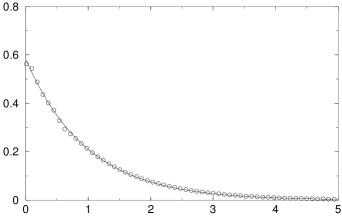
Figure 3.1: $E\times t$ for different lattice spacings and $\eta=0$ (above) and $E\times t$ for $N=1000$ and $\eta=1$ (below). The linear dimension is fixed at $L=1$.

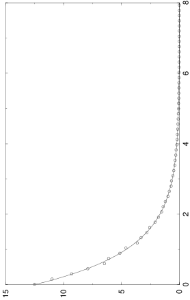
Figure 3.2: $E\times t$ for $\eta=0$ and various $N$ (above) and $E\times t$ for $\eta=1$ and $N=200$ (below). The dimensions of the membrane are $L\times L=1$ for all runs.

Figure 3.1 shows some results for the conditions of the previous section for various parameters. Notice the improvement of energy conservation for finer resolutions and the very good exponential fitting for $\eta=1$. This exponential result is expected, since the vibrating string could be understood in terms of the Fourier space, where each mode behaves as a decoupled harmonic oscillator with a damping given by $\eta$.

3.2 The Membrane (2D)

These simulations were also executed in a PC of $350MHz$, and for lattices of $N=500$ the integration time reached half an hour.

Figure 3.2 shows some results for $\eta=0$ and $\eta=1$. For a non-conservative system ($\eta=1$), we see also the exponential fitting for $N=200$.

Appendix A Taylor’s Theorem

A.1 Definitions

When we want to transform a differential equation into a difference equation, the Taylor expansion is often used:

$$f(x) = f(x_{0})+f^{\prime}(x_{0})(x-x_{0})+\frac{1}{2}f^{\prime\prime}(x_{0})(x-x_{0})^{2}+...=$$ (A.1)

$$= \sum^{\infty}_{n=0}\frac{f^{(n)}(x_{0})}{n!}(x-x_{0})^{n},$$ (A.2)

where $x_{0}$ is the point around which we want to expand $f(x)$. An alternative form for this expansion is achieved doing a simple variable change $x\rightarrow x+h$ and $x_{0}\rightarrow x$:

$$f(x+h)=\sum_{n=0}^{\infty}\frac{f^{(n)}(x)}{n!}h^{n}$$ (A.3)

In the numerical case we will be interested in truncating the series, so that we finish with a finite number of terms. We could then write this expansion in the following form:

$$f(x+h)=\sum_{n=0}^{m}\frac{f^{(n)}(x)}{n!}h^{n}+{\cal O}(h^{m+1}),$$ (A.4)

where ${\cal O}(h^{m+1})$ corresponds to the truncated terms which powers of $h$ are equal or higher than $m+1$ (this term is frequently called the error of order $m+1$). Notice that under the numerical point of view it is important to know the order of ${\cal O}$ in the discretization, since for $h\ll 1$, the greater the order of ${\cal O}$ the more negligible will be the error.

A.2 Useful Expansions

Some expansions that will be used throughout this text are shown below. All of them could be obtained from (A.4) by directly solving for the desired term or using more than one expansion to find higher order expansions for the derivative, and then solving the system. For instance:

$$\left\{\begin{array}[]{cc}f(x+h)&=f(x)+f^{\prime}(x)h+\frac{1}{2}f^{\prime\prime}(x)h^{2}+...\\ f(x-h)&=f(x)-f^{\prime}(x)h+\frac{1}{2}f^{\prime\prime}(x)h^{2}-...\end{array}\right.$$

$$f^{\prime}(x)=\frac{f(x+h)-f(x)}{h}-{\cal O}(h)$$ (A.5)

$$f^{\prime}(x)=\frac{f(x+h)-f(x-h)}{2h}-2{\cal O}(h^{2})$$ (A.6)

$$f^{\prime\prime}(x)=\frac{f(x+h)-2f(x)+f(x-h)}{h^{2}}-2{\cal O}(h^{2})$$ (A.7)

$$\frac{\partial f(x,y)}{\partial x}=\frac{f(x+h,y)-f(x,y)}{h}-{\cal O}(h)$$ (A.8)

$$\frac{\partial^{2}f(x,y)}{\partial x^{2}}=\frac{f(x+h,y)-2f(x,y)+f(x-h,y)}{h^{2}}-2{\cal O}(h^{2})$$ (A.9)

Notice that when we divide an error of order ${\cal O}(h^{n})$ by $h^{r}$, automatically this error turns to order $n-r$, i.e., ${\cal O}(h^{n})/h^{r}={\cal O}(h^{n-r})$.

Bibliography

- [1] M. Gleiser and R. O. Ramos, Phys. Rev. D50, 2441 (1994).
- [2] G. Aarts and J. Smit, Nucl. Phys. B555, 355 (1999); Phys. Rev. D61, 025002 (2000).
- [3] For a good review on the subject and its high-energy counterpart, see D. Boyanovsky and H. J. de Vega, “Dynamics of Symmetry Breaking Out of Equilibrium: From Condensed Matter to QCD and the Early Universe”, hep-ph/9909372.
- [4] J. Borrill and M. Gleiser, Nucl. Phys. B483, 416 (1997)
- [5] G. B. Arfken, H. J. Weber, Mathematical Methods for Physicists, 4th Ed.
- [6] W. H. Press et al., Numerical Recipes, 2nd Ed.
- [7] K. R. Symon, Mechanics, 3rd. Ed.
- [8] W. Cheney e D. Kincaid, Numerical Mathematics and Computing, 3rd Ed.
- [9] A. R. Mitchell e D. F. Griffiths, The Finite Difference Method in Partial Differential Equations