Efficiency of different numerical methods for solving Redfield equations

Abstract

The numerical efficiency of different schemes for solving the Liouville-von Neumann equation within multilevel Redfield theory has been studied. Among the tested algorithms are the well-known Runge-Kutta scheme in two different implementations as well as methods especially developed for time propagation: the Short Iterative Arnoldi, Chebyshev and Newtonian propagators. In addition, an implementation of a symplectic integrator has been studied. For a simple example of a two-center electron transfer system we discuss some aspects of the efficiency of these methods to integrate the equations of motion. Overall for time-independent potentials the Newtonian method is recommended. For time-dependent potentials implementations of the Runge-Kutta algorithm are very efficient.

I Introduction

Besides classical and semi-classical descriptions of dissipative molecular systems several quantum theories exist which fully account for the quantum effects in dissipative dynamics. Among the latter are the reduced density matrix (RDM) formalism [1, 2, 3, 4, 5] and the path integral methods [6, 7]. Here we concentrate on the Redfield theory [8, 9], in which one has to solve a master equation for the RDM. It is obtained by performing a second order perturbation treatment in the system-bath coupling as well as restricting the calculation to the Markovian limit. With this approach the quantum dynamics of an “open” system, e.g., the exchange of energy and phases with the surroundings modeled as a heat bath, can be described. The unidirectional energy flow into the environment is called dissipation. Within this theory it is possible e.g. to simulate the dissipative short-time population dynamics usually detected by modern ultrafast spectroscopies.

Because the Redfield theory is a Markovian theory the time evolution of the RDM is governed by equations containing no memory kernel. In the original Redfield theory [8, 9] the secular approximation was performed. In this approximation it is assumed that every element of the RDM in the energy representation is coupled only to those elements that oscillate at the same frequency. In the present study we do not perform this additional approximation.

For larger systems numerical implementations for solving the Redfield equation are numerically very demanding and therefore require that one finds the most appropriate way to perform the time evolution of the RDM. Straightforward one can construct and directly diagonalize the Liouville superoperator. For processes with a time-independent Hamiltonian the rates, i.e. the characteristic inverse times of an exponential decay of the occupation probability of the excited states, can be obtained in this way. In such an approach a huge number of floating point operations will be involved and the overall computational effort will scale as ${\cal N}^{6}$ where ${\cal N}$ is the size of the basis of vibronic states. Furthermore the direct diagonalization can be numerically unstable, but nevertheless has been successfully used (see e.g. [10]). Another strategy suggests solving ${\cal N}^{2}$ ordinary differential equations and requires products between the Liouville superoperator and the RDM which scale as ${\cal N}^{4}$ (see e.g. [11]). This is also numerically demanding for larger systems. Assuming a bilinear system-bath coupling the numerical effort can be reduced considerably by rewriting the Redfield equation in such a form that only matrix-matrix multiplications are needed [12] rather than applying a superoperator onto the RDM. Hence, a computational time scaling of ${\cal N}^{3}$ and a storage requirement of ${\cal N}^{2}$ is achieved. In the present paper our numerical studies will be based on this approach.

If one wants to reduce the scaling of the numerical effort with increasing number of basis functions even more one has to go to stochastic wave function methods [13, 14, 15, 16]. They prescribe certain recipes to unravel the Redfield equation and to substitute the RDM by a set of wave functions which evolve partially stochastically in time. The method will have the typical scaling of the well developed and optimized wave function propagators, i.e. ${\cal N}^{2}$. It has been applied, for example, to electron transfer systems [17, 18, 19] and shown to give accurate results. Direct solutions and the stochastic wave packet simulations have already been compared numerically [20, 21]. All these first studies were restricted to dissipation operators with Lindblad form [22]. Breuer et al. [23] showed that the stochastic wave function approach can also be applied to Redfield master equations without the secular approximation and for non-Markovian quantum dissipation. In particular for complex systems with a large number of levels its practical application is very advantageous. Between the direct and the stochastic methods to solve the Redfield equation the accuracy differs especially because direct RDM integrators are numerically “exact” while the stochastic wave function simulation methods have statistical error. The scope of this work are small and medium size problems. Therefore we compare the different numerical algorithms for a direct integration of the Redfield equation. But when using stochastic methods for density matrix propagation one has to solve Schrödinger-type equations with a non-Hermitian Hamiltonian. For that purpose the same algorithms as investigated here can be used. In this sense the present study is also of importance for solving Redfield equations by means of stochastic methods.

Here we use different numerical schemes to solve the Liouville-von Neumann equation. The performance of the well-known Runge-Kutta (RK) scheme is studied in two different implementations: as given in the Numerical Recipes [24] and by the Numerical Algorithms Group [25]. Compared to these general-purpose solvers are more special algorithms which have been applied previously to the time evolution of wave packets and density matrices. For density matrices these are the Short-Iterative-Arnoldi (SIA) propagator [12, 26], the short-time Chebyshev polynomial (CP) propagator [11], and the Newtonian polynomial (NP) propagator [27, 28]. The latter propagator is also used as a reference method because of its high accuracy. In addition, a symplectic integrator (SI), which was originally developed for solving classical equations of motion and extended to wave packet[29, 30] and density matrix propagation [31], is tested.

Besides the propagation algorithm one has to determine the appropriate representation in which to calculate the elements of the RDM and the Liouville superoperator. The choice depends strongly on the type of physical problem that one considers. Coordinate (grid) representation has an advantage when dealing with complicated potentials, e.g. non-bonding potentials. For the problem of dissociation dynamics in the condensed phase the grid representation has been applied based on a Lindblad-type master equation [32]. Other examples using grids are works of Gao [33] and Berman et al. [27]. Convenient treatment of electron transfer dynamics is done in state representation, because one can model the system using a set of harmonic diabatic potentials [34]. Other authors [12, 35, 36] choose the adiabatic eigenstates of the whole system as a basis set to treat similar problems. A comparative analysis of the benefits and drawbacks of the diabatic and adiabatic representation in Redfield theory will be given elsewhere [37]. From the viewpoint of numerical efficiency we focus on both representations in the present article.

The paper is organized as follows. In the next section we will make a short introduction to the model system and a discussion on the versions of the Redfield equation and the numerical scaling that they exhibit. In Section III the methods for propagation used in this work are briefly reviewed. In Section IV we compare the efficiency of several propagators in solving a simple electron transfer problem with multiple levels. A summary is given in the last section.

II The Redfield equation and its scaling properties

In the RDM theory the full system is divided into a relevant system part and a heat bath. Therefore the total Hamiltonian consists of three terms – the system part $H_{\rm S}$, the bath part $H_{\rm B}$ and the system-bath interaction $H_{\rm SB}$:

$$H=H_{\rm S}+H_{\rm B}+H_{\rm SB}.$$ (1)

The separation into system and bath allows one to formulate the system dynamics, described by the Liouville-von-Neumann equation, in terms of the degrees of freedom of the relevant system. In this way one loses the mostly unimportant knowledge of the bath dynamics but gains a great reduction in the size of the problem. Such a reduction together with a second order perturbative treatment of the system-bath interaction $H_{\rm SB}$ and the Markov approximation leads to the Redfield equation [8, 9, 1, 2]:

$$\dot{\rho}=-\frac{i}{\hbar}[H_{\rm S},\rho]+{\cal R}\rho={\cal L}\rho.$$ (2)

In this equation $\rho$ denotes the reduced density operator and ${\cal R}$ the Redfield tensor. If one assumes bilinear system-bath coupling with system part $K$ and bath part $\Phi$

$$H_{\rm SB}=K\Phi$$ (3)

one can take advantage of the following decomposition [12, 2]:

$$\dot{\rho}=-\frac{i}{\hbar}\left[H_{\rm S},\rho\right]+\frac{1}{\hbar^{2}}\{\left[\Lambda\rho,K\right]+\left[K,\rho\Lambda^{\dagger}\right]\}.$$ (4)

Here the system part $K$ of the system-bath interaction and $\Lambda$ together hold equivalent information as the Redfield tensor ${\cal R}$. The $\Lambda$ operator can be written in the form

$$\Lambda=K\int\limits_{0}^{\infty}d\tau\langle\Phi(\tau)\Phi(0)\rangle e^{i\omega\tau}=KC(\omega)~{}.$$ (5)

The two-time correlation function of the bath operator $C(\tau)=\langle\Phi(\tau)\Phi(0)\rangle$ and its Fourier-Laplace image $C(\omega)$ can be relatively arbitrarily defined and depend on a microscopic model of the environment. Different classical and quantum bath models exist. Here we take a quantum bath [26], i.e. a large collection of harmonic oscillators in equilibrium, that is characterized by a Bose-Einstein distribution and a spectral density $J(\omega)$:

$$C(\omega)=2\pi\left[1+\left(e^{\hbar\omega/k_{B}T}-1\right)^{-1}\right]\left[J(\omega)-J(-\omega)\right]~{}.$$ (6)

Now we look for bases that span the degrees of freedom of the relevant system. Let us consider atomic or molecular centers $m$ at which the electronic states $|m\rangle$ of the system are localized. Their potential energy surfaces (PESs) will be approximated by harmonic oscillator potentials, displaced along the reaction coordinate $q$ of the system. As such a coordinate one can, for example, choose a normal mode of the relevant system part which is supposed to be strongly coupled to the electronic states. The centers are coupled to each other with constant coupling $v_{mn}$. For example two such coupled centers are sketched in Fig. 1. The coupled surfaces $|1\rangle$ and $|2\rangle$ are assumed to describe excited electronic states. The electron transfer takes place after an excitation of the system from its ground state $|\mbox{g}\rangle$.

Using this microscopic concept we define $K$ as the system’s coordinate operator

$$K=q=\sum\limits_{m}\left(2\omega_{m}{\cal M}/\hbar\right)^{-1/2}\left(a_{m}^{\dagger}+a_{m}\right)|m\rangle\langle m|~{}$$ (7)

where $a_{m}$ and $a_{m}^{\dagger}$ are the boson operators for the normal modes at the center $m$, ${\cal M}$ is the reduced mass and $\omega_{m}$ are the eigenfrequencies of the oscillators. In the same picture the Hamiltonian of the relevant system reads

$$H_{\rm S}=\sum\limits_{mn}\{\delta_{mn}\left[U_{m}+\left(a_{m}^{\dagger}a_{m}+\frac{1}{2}\right)\hbar\omega_{m}\right]+\left(1-\delta_{mn}\right)v_{mn}\}|m\rangle\langle n|~{}.$$ (8)

From this point on we consider two possible state representations in order to calculate the matrix elements of $\rho$ and the operators $H_{\rm S}$, $K$ and $\Lambda$. The diabatic (local) basis is a direct product of the eigenstates $|M\rangle$ of the harmonic oscillators and the relevant electronic states $|m\rangle$ (Fig. 1, left panel). The intercenter coupling $v_{mn}$ gives rise to off-diagonal elements of the Hamiltonian matrix

$$\langle mM|H_{\rm S}|nN\rangle=\left[U_{m}+\left(M+\frac{1}{2}\right)\hbar\omega_{m}\right]\delta_{mn}\delta_{MN}+\left(1-\delta_{mn}\right)v_{mn}\langle mM|nN\rangle~{},$$ (9)

where $U_{m}$ are the energies of the minima of the diabatic PESs. Other important properties of the diabatic representation are the equidistance in the level structure and the diagonal form of the system-bath interaction operator $H_{\rm SB}$. This determines the tridiagonal band form of the operator $K$.

When neglecting the influence of the intercenter coupling on the dissipation a very efficient numerical algorithm can be derived [38, 34]. Of course, for strong intercenter couplings the populations $\langle mM|\rho|mM\rangle$ at long times deviate from their expected equilibrium values. But even for very small couplings there are cases in which the population does not converge to its equilibrium value [37]. Therefore this neglect of the influence of the intercenter coupling on the dissipation has to be handled with care. On the other hand this approximation makes the extension of the present electron transfer model to many modes conceptually much easier [17, 18].

The matrix elements of the operators in the dissipative part of Eq. (4) read

$$\langle mM|K|nN\rangle=\left(2\omega_{m}{\cal M}/\hbar\right)^{-1/2}\delta_{mn}\left(\delta_{M+1,N}\sqrt{M+1}+\delta_{M-1,N}\sqrt{M}\right)$$ (10)

and

$$\langle mM|\Lambda|nN\rangle=\langle mM|K|nN\rangle C(\omega_{mMnN})~{}.$$ (11)

In Eq. (11) $\omega_{mMnN}$ denote the transition frequencies of the system

$$\hbar\omega_{mMnN}=\langle mM|H_{\rm S}|mM\rangle-\langle nN|H_{\rm S}|nN\rangle.$$ (12)

Since the system can emit or absorb only at the eigenfrequencies of the system oscillators $\omega_{m}$ the spectral density of the bath $J(\omega)$ is effectively reduced to a few discrete values $J(\omega)=\sum_{m}\gamma_{m}\delta(\omega-\omega_{m})$. The advantage of this approach lies in the scaling behavior with the number of basis functions. As shown in Fig. 2 it scales like ${\cal N}^{2.3}$ where ${\cal N}$ is the number of basis functions. This is far better than the scaling without neglecting the influence of the intercenter coupling on the dissipation as described below.

If the system Hamiltonian $H_{\rm S}$ is diagonalized it is possible to use its eigenstates as a basis (Fig. 1, right panel), in which to calculate the elements of the operators in Eq. (4). Of course there will be no longer any convenient structure in $K$ or $\Lambda$, so that the full matrix-matrix multiplications are inevitable. For this reason the computation of ${\cal L}\rho(t)$ scales as ${\cal N}^{3}$, where ${\cal N}$ is the number of eigenstates of $H_{\rm S}$. There appears to be a minimal number ${\cal N}_{0}$ below which the diagonalization of $H_{\rm S}$ fails or the completeness relation for $|mM\rangle$ is violated. Nevertheless, the benefit of this choice is the exact treatment of the system-bath interaction. Denoting the unitary transformation that diagonalizes $H_{\rm S}$ by $U$ one has

$${\bf\epsilon}=U^{\dagger}H_{\rm S}U$$ (13)

where ${\bf\epsilon}$ is a diagonal matrix containing the eigenvalues. In this way it is straightforward to obtain the matrices for $\rho$ and $K$. Equation (6) for $C(\omega)$ still holds but a new definition of the spectral density $J(\omega)$ is necessary because of the non-equidistant adiabatic eigenstates. The bath absorbs over a large region of frequencies and this is characterized in the model by $J(\omega)$. One needs the full frequency dependence of $J(\omega)$ which we take to be of Ohmic form with exponential cut-off:

$$J(\omega)=\eta\Theta(\omega)\omega e^{-\omega/\omega_{c}}.$$ (14)

Here $\Theta$ denotes the step function and $\omega_{c}$ the cut-off frequency. In this study all system oscillators have the same frequency $\omega_{1}$ (see Table I) and the cut-off frequency $\omega_{c}$ is set to be equal to $\omega_{1}$. The normalization prefactor $\eta$ is determined such that

$$\int\limits_{0}^{\infty}d\omega J(\omega)=\gamma_{1}~{}.$$ (15)

Equation (14) together with Eq. (6) yields the correlation function in adiabatic representation.

The introduced representations allow us to consider the numerical effort for a single computation of the right hand side of Eq. (4), i.e. of ${\cal L}\rho(t)$. In the diabatic representation its computation can be approached using two different algorithms. It is possible to perform matrix-matrix multiplication only on those elements of $K$ and $\Lambda$ which have nonzero contributions to the elements of ${\cal L}\rho(t)$ (Fig. 2, solid line). This is advantageous because of the tridiagonal form of $K$ in diabatic representation and shows the best scaling properties, namely ${\cal N}^{2.3}$. In the same representation but performing the full matrix-matrix multiplications in Eq. (4) (Fig. 2, dashed line) the scaling behavior is slightly worse than the same operation in adiabatic representation (Fig. 2, dotted line). This is due to the non-diagonal Hamiltonian $H_{\rm S}$ in the former case that makes the computing of the coherent term (see Eq. (2)) more expensive. Below we will take the full matrix-matrix multiplication to evaluate ${\cal L}\rho(t)$ in both representations. We do this to concentrate on the various propagation schemes, not the unequal representations. Nevertheless there are performance changes in the different representations because of the disparate basis functions and forms of the operators in these basis functions.

III The different propagation schemes

A Runge-Kutta method

The RK algorithm is a well-known tool for solving ordinary differential equations. Thus, this method can be successfully applied to solve a set of ordinary differential equations for the matrix elements of Eq. (4). It is based on a few terms of the Taylor series expansion. In the present work we use the FORTRAN77 implementation as given in the Numerical Recipes [24] which is a fifth-order Cash-Karp RK algorithm and will be denoted as RK-NR. As alternative the RK subroutine from the Numerical Algorithms Group [25] which is based on RKSUITE [39] was tested with a 4(5) pair. It will be referred to as RK-NAG. Both RK-NAG and RK-NR involve terms of fifth order and use a prespecified tolerance $\tau$ as an input parameter for the time step control. The tolerance $\tau$ and the accuracy of the calculation are not always simply proportional. Usually decreasing $\tau$ results in longer CPU times.

In our previous work [40] a time step control mechanism different from those used in RK-NAG and RK-NR was tested. Discretizing the time derivative in Eq. (2) and requiring

$$\left|\frac{\rho(t_{i+1})-\rho(t_{i})}{\Delta t}+{\cal L}\rho(t_{i})\right|<\tau$$ (16)

one only has to call the propagation subroutine once and to store the previous RDM. In addition one has to calculate the action of the Liouville superoperator ${\cal L}$ onto the RDM but the numerical effort for this is small compared to a call of the propagation subroutine. It was shown in Ref. [40] that this time step control is the most efficient for propagation with the coherent terms in Eq. (2) only but disadvantageous for problems with dissipation. This is the reason why we do not include this algorithm in the present study.

B Short Iterative Arnoldi propagator

The SIA propagator [12, 26] is a generalized version of the Short Iterative Lanczos propagator [41] to non-Hermitian operators. With the Short Iterative Lanczos algorithm the wave function can be propagated by approximating the time evolution operator in Krylov space, which is generated by consecutive multiplications of the Hamiltonian on the wave function. In analogy the Krylov space within the SIA method is constructed by recursive applications of the Liouville superoperator onto the RDM $\rho_{n}={\cal L}^{n}\rho(t)$. In this way it is tailored for the RDM at every moment in time. The Liouville superoperator, denoted by $l$ in Krylov space, has Hessenberg form

$${\bf{\cal L}}\approx{V}lV^{\rm T}~{},$$ (17)

where the orthogonal transformation matrix $V$ is constructed iteratively using the so-called Lanczos procedure [12]. The Krylov representation $l$ can be easily diagonalized to $L$ with the help of a transformation matrix $S$:

$$e^{{\cal L}t}\approx VSe^{Lt}S^{-1}V^{\rm T}~{}.$$ (18)

Since the diagonalization is performed in the Krylov space the numerical effort depends on its dimension which can be chosen small in practice. Having thus derived a diagonal operator $e^{{L}t}$ the calculation of $\rho(t)$ is straightforward.

C Symplectic integrator

The SIs were originally developed for solving classical equations of motion [42]. The time evolution of a classical Hamiltonian system can be viewed as a canonical transformation and SIs are sequences of canonical transformations. Recently it was shown that the time evolution of wave packets [29, 30] and density matrices [31] can also be performed using SIs. In order to rewrite the Redfield equations in the form of coupled canonical variables that are analogous to classical equations of motion one defines the functions[31]

$$Q(t) = \rho(t)~{},$$ (19)

$$P(t) = \dot{\rho}(t)~{},$$ (20)

the operator

$$W = -\frac{1}{\hbar^{2}}{\cal L}^{2}~{},$$ (21)

and the Hamiltonian function

$$G(Q,P)=\frac{1}{2}[P^{T}P+Q^{T}WQ]~{}.$$ (22)

Doing so one obtains equations of motion analogous to the classical ones

$$\frac{d}{dt}P(t) = -\frac{\partial G(Q,P)}{\partial Q}=-WQ(t)~{},$$ (23)

$$\frac{d}{dt}Q(t) = \frac{\partial G(Q,P)}{\partial P}=P(t)~{}.$$ (24)

Rewriting this into the SI algorithm of order $m$ yields [31]

$$P_{i}=P_{i-1}+\frac{b_{i}\Delta t}{\hbar^{3}}{\cal L}^{2}Q_{i-1}$$ (25)

$$Q_{i}=Q_{i-1}+\frac{a_{i}\Delta t}{\hbar}P_{i}$$ (26)

for $i=1,\ldots,m$. Different sets of coefficients $\{a_{i}\}$ and $\{b_{i}\}$ are given in the literature. Here we choose the McLachlan-Atela fourth-order method [43]. The coefficients for this method are listed in Ref. [44]. A comparison of the McLachlan-Atela fourth-order method with the McLachlan-Atela third-order method [43] and Ruth’s third-order method [42] has been given elsewhere [31].

D Newton polynomial scheme

Another way to solve Eq. (2) is by a polynomial expansion of the time-evolution operator. Such methods are well established and approved for wave-function propagation [41, 28]. Recently the Faber [45] and NP [27] algorithms have been applied to propagate density matrices and it has been shown that they behave very similarly [45]. The main idea of the NP method is the representation of the Liouville superoperator by a polynomial interpolation

$$e^{{\cal L}t}\approx{\cal P}_{N_{p}-1}({\cal L})\equiv\sum\limits_{n=0}^{N_{p}-1}a_{n}\rho_{n}=\sum\limits_{n=0}^{N_{p}-1}a_{n}\prod\limits_{j=0}^{n-1}({\cal L}-\lambda_{j})$$ (27)

of order $N_{p}$ where the $\rho_{n}$ are computed recursively and $a_{n}$ are the $n$-th divided differences. The interpolation points $\lambda_{j}$ can be chosen to form a rectangular area in the complex plane (see Fig. 3) which contains all eigenvalues of ${\cal L}$. This interpolation scheme is uniform, i.e., the accuracy in energy space is approximately the same in the whole spectral range of ${\cal L}$. This is in contrast to schemes such as the SIA propagator which are nonuniform approximations. A consequence of this property is the very high accuracy which can be achieved with uniform propagators. This is why we take a high-order NP expansion as reference solution. Since the quality of the approximation of the time evolution operator is equivalent to a scalar function with the same interpolation points $\lambda_{j}$, one can, before performing the actual calculation, check the accuracy on a scalar function. For the calculation with the NP propagator we set the truncation limit of the expansion to $10^{-15}$, i.e., the sum in Eq. (27) is truncated when the residuum fulfills $a_{n}||\rho_{n}||<10^{-15}$ [28].

E Chebyshev polynomial scheme

As a last contribution to the present study we will examine the CP propagator. Recently it was studied by Guo et al. [11] for density matrices. The Liouville superoperator is approximated by a series of CPs $T_{k}(x)$. Generally the CPs diverge for non-real arguments. For propagators of the kind $e^{-iHt}$ it has been shown [28] that the CPs may tolerate some imaginary part in the eigenvalues of $H$. The stability region has the form of an ellipse with a center at the origin and a very small half-axis in imaginary directions [28]. In contrast, the eigenvalues of the Liouville superoperator are spread over the negative real half of the complex plane and symmetrically with respect to the real axis (see Fig. 3). The real components for the system that we consider are one order of magnitude smaller than the imaginary components. This is why we make the expansion along the imaginary axis and use an expression similar to that already applied to wave function propagation [41]:

$$e^{{\cal L}t}\approx e^{L^{+}\Delta t}\sum\limits_{n=0}^{N_{p}-1}(2-\delta_{n0})J_{n}(L^{-}\Delta t)T_{n}({\tilde{L}})~{}.$$ (28)

Here the expansion coefficients $J_{n}$ are the Bessel functions of the first kind, and ${\tilde{L}}$ is the appropriately scaled Liouville superoperator: ${\tilde{L}}=({\cal L}-L^{+})/L^{-}$, where $L^{-}$ and $L^{+}$ are the half span and the middle point of the spectrum of ${\cal L}$. Since the spectrum is symmetric with respect to the real axis, $L^{+}=0$. The time evolution of $\rho$ is given by

$$\rho(t+\Delta t)\approx\sum\limits_{n=0}^{N_{p}-1}(2-\delta_{n0})J_{n}(L^{-}\Delta t){\tilde{\rho}}_{n}~{}.$$ (29)

The Chebyshev vectors ${\tilde{\rho}}_{n}$ are generated by means of a recurrence procedure:

$${\tilde{\rho}}_{n}=2{\tilde{L}}{\tilde{\rho}}_{n-1}+{\tilde{\rho}}_{n-2},\mbox{~{}~{}}{\tilde{\rho}}_{0}=\rho(t)\mbox{~{}and~{}}{\tilde{\rho}}_{1}={\tilde{L}}{\tilde{\rho}}_{0}~{}.$$ (30)

For the CP and NP methods one has to adjust the values of the spectral parameters $L^{-}$ and $L^{+}$. One can obtain some knowledge about the spectrum of ${\cal L}$ by an approximate diagonalization, e.g. by Krylov subspace methods. For instance, Fig. 3 shows an approximate spectrum of ${\cal L}$ appropriately scaled so that all eigenvalues lie within the rectangle formed by the Newtonian interpolation points.

IV Performance of propagation methods

The aim of this section is to compare the different numerical methods described above for propagating the RDM in time. The calculations were performed for both RK methods with different tolerance parameters $\tau$ and for the SI as well as the NP, CP, SIA propagators with different timesteps. The number of expansion terms $N_{p}$ in NP and CP propagators is 170 and 64, respectively. The dimension of the Krylov space for the SIA method was set to 12 because smaller as well as larger values are less efficient for the example studied here. All computations were made on Pentium III 550 MHz personal computers with intensive use of BLAS and LAPACK libraries. The code was compiled using the PGF90 Fortran compiler [46]. For estimation of the computational error of all methods the NP algorithm with 210 terms was chosen as a benchmark.

In this work we consider only two centers $m=1,2$ which is the minimal model to describe the main physics of an electron transfer reaction. A basis size of 16 levels per center satisfies the completeness relation and presents no difficulties during the diagonalization of $H_{\rm S}$. The electronic coupling was $v_{12}=0.1$ eV. We choose $\gamma_{1}=\gamma_{2}=1.57863\times{}{\rm 10^{-2}~{}eV}{\rm\AA{}^{-2}}$ and ${\cal M}=20m_{p}$ where $m_{p}$ is the proton mass. The temperature $T=298$ K is used. In Table I the parameters for the system oscillators are given.

The process that is simulated involves the following scenario. A Gaussian wave packet is prepared as initial state by a vertical transition from the lowest vibrational level of the ground electronic state $|{\rm g}\rangle$ to the first (upper) center $|1\rangle$:

$$\rho_{1M1N}(t=0)=\langle 1M|{\rm g}0\rangle\langle{\rm g}0|1N\rangle~{}.$$ (31)

The energy distribution of the occupied eigenstates by the wave packet depends on the displacement $q^{0}_{\rm g}-q^{0}_{1}$ between the PESs of $|{\rm g}\rangle$ and $|1\rangle$. During the pulse the two excited electronic states $|1\rangle$ and $|2\rangle$ are assumed to be decoupled. In this way one can simulate the absorption of electromagnetic radiation from a pulse with vanishing width. Right after the pulse is over, the wave packet starts moving on the excited PESs and spreading. The relevant system part begins losing energy to the bath and dephasing. The population on the upper center starts decaying. When the damping is not too strong, as for the model parameter studied here, a damped oscillation of the population between the two excited PESs can be seen. We assume no coupling to the ground state after the pulse. After a certain time the system reaches its equilibrium state.

In all cases the RDM was propagated for a total time period of $3\times{}10^{5}$ a.u. which is sufficient for complete relaxation to equilibrium. It was compared to the RDM $\rho_{\rm ref}$ evaluated by the NP algorithm at the same points in time. The relative error $\varepsilon(t)$ of each method at a certain moment in time $t$ has been estimated using a formula similar to that proposed for wave functions by Leforestier et al.[41]:

$$\varepsilon(t)=\left|1-\frac{{\rm Tr}\left(\rho(t)\rho_{\rm ref}(t)\right)}{{\rm Tr}\left(\rho^{2}_{\rm ref}(t)\right)}\right|~{}.$$ (32)

As the error $\varepsilon$ we define the maximum value of $\varepsilon(t)$ over the total propagation time. For more details we refer to our previous paper [40]. Other error measures (see for example [47, 11]) can be used as well but they will have the same qualitative behavior.

As an index for the numerical effort two possibilities were explored. The first one is a direct measurement of the CPU time of the total propagation (Fig. 4). It may look quite different on other computer architectures or even on the same architecture but under changed operation conditions. An evidence of the performance (Fig. 4) will be expressed by means of CPU time versus the error $\varepsilon$.

Another approach to describe the numerical effort has been proposed [11] and is called efficiency factor. It is defined as the ratio between the timestep $\Delta t$ and the number of operations ${\cal L}\rho(t)$ within this timestep. Because of the definition it is a machine independent quantity. The larger the efficiency factor, the better the performance of the algorithm. Because the RK algorithms propagate with variable timestep we cannot directly use the definition of the efficiency factor. Instead we define a quantity $\alpha$ as the total number $N_{c}$ of ${\cal L}\rho(t)$-evaluations divided by the total time for the propagation:

$$\alpha=N_{c}/(N_{s}\overline{\Delta t})~{}.$$ (33)

Here $N_{s}$ denotes the total number of timesteps. The inverse of $\alpha$ will have the meaning of an efficiency factor for an averaged timestep $\overline{\Delta t}$. We should point out that $N_{c}$ does not take into account the effort for summation of the different contributions. In particular in the case of the NP method the summation of the different terms in the polynomial expansion Eq. (27) can be non-negligible. This can be seen in the different relative performance of the propagators shown in Figs. 4 and 5. We consider both the CPU time and the quantity $\alpha$ as measures of the numerical effort.

Contributions from the algorithm to calculate ${\cal L}\rho(t)$ also influence the CPU time. As discussed above, in all computations represented in Figs. 4 and 5 the full matrix-matrix multiplications in Eq. (4) were performed. The performance of the CP, NP, SI and SIA methods is only influenced very little by the choice between diabatic and adiabatic representation. Both RK implementations are less efficient in the adiabatic than in the diabatic representation, though the RK-NAG scheme has still the best performance besides the NP algorithm. The RK-NR scheme has an advantage for computation in diabatic rather than in adiabatic representation especially for medium precision requirements. In that range the performance curves of the RK methods exhibit a shoulder for the adiabatic case which seems to result from a numerical artifact.

Because the error of the SIA algorithm is not uniformly distributed in energy space [48] we could expect some difference in its performance in diabatic and adiabatic representation. But because the coupling $v_{12}$ chosen here is not very large, the eigenstates of the coupled system are just slightly disordered (see Fig. 1, right plot) and hence the performance of the SIA algorithm is almost not changed.

The uniformity, stability and high accuracy of the CP propagator for wave functions is well known [41, 48, 47]. The CP approach to density matrix propagation was introduced by Guo and Chen [11]. Using a damped harmonic oscillator as model system and starting from a pure state they established that the relative error can reach the machine precision limits ($10^{-15}$) for sufficiently small stepsize. However, for the system of coupled harmonic potentials studied here and using an initial RDM with non-zero off-diagonal elements the error saturates at $\varepsilon\approx 10^{-8}$ (see Fig. 4). It was not possible to decrease this saturation limit of $\varepsilon$ neither by increasing the order of the CP nor by decreasing the timestep. This saturation limit seems to depend strongly on the imaginary part of the eigenvalues of ${\cal L}$. For large timesteps the CP method loses its stability and one needs to estimate the efficiency range of $N_{p}$, $\Delta t$ and $L^{-}$. Turning off the dissipation we could reach much higher accuracy with the CP propagator as expected.

The SI is easy to implement. The expansion coefficients are fixed and can be taken from literature. At the same time the fixed coefficients seem to limit the accuracy. For not too high accuracy the performance of the SI is as good as that of the other propagators in adiabatic representation. In diabatic representation its performance is a little worse. But we were not able to achieve very high accuracy with this method. This might be due to the special version, the fourth order McLachlan-Atela method, which we chose.

As already highlighted [45] the NP scheme is very stable for arbitrary spectral properties of ${\cal L}$. The only restriction is that the spectrum must be confined within the area formed by the interpolation points. In our investigation the NP propagator performs with a good accuracy for timesteps of 1500 a.u. ($N_{p}=170$) which is 10 times larger than the step size of the CP scheme. Higher order expansions might be even more efficient but the numerical implementation gets tricky and easily unstable. For timesteps of 100 a.u. and $N_{p}=50$ the NP algorithm is already numerically exact but computational very expensive (see the arrows in Fig. 4 and Fig. 5). For problems with time-dependent Hamiltonians (e.g. non-stationary external fields with relatively small amplitude) the RK and SIA methods will be more efficient with small timestep.

At the end we should point out that there exists no ultimate method to determine the performance of a certain numerical approach which could be valid for different platforms. Tuning and optimization features are generally not portable and this may cause even different scaling behavior and hence a different method of preference. That is the reason why the generality of the results is limited to similar computation platforms and even to systems with similar properties of the corresponding Liouville superoperator. But on the other hand this study can give hints on the performance of the different algorithms in general.

V Summary

In the present work an estimation of the numerical efficiency of several methods for density matrix propagation has been given. The example of electron transfer in a two-center system has been used for this purpose. A specific measure of the numerical effort has been introduced in order to compare methods with fixed timestep and such ones with timestep control (RK). Besides the method of reference (NP) the RK-NAG approach shows best performance for both cases of adiabatic and diabatic representation. The advantage of the SIA propagator is that the accuracy improves with decreasing the timestep in all cases we investigated. That is not the case with the CP propagator which exhibits a saturation of accuracy and is therefore not convenient for very small timesteps. The easy-to-implement SI gives reasonable performance for not too high accuracy. The present SI seems to be limited in accuracy due to the fixed coefficients.

The present studies were restricted to state bases. Of course similar calculations can be done on a grid which is especially useful for complicated or unbound potentials. In these cases another propagator, the split operator [49], should be taken into account. This operator has the advantage that its performance does not (directly) depend on the spectral range of the Hamiltonian or Liouville operator. So it may perform very well for problems with a large spectral range although it cannot be applied to operators which have mixed terms in coordinate and momentum operators. The use of the mapped Fourier method [50] may reduce the number of grid points significantly and first wave packet propagations with this method have been done [51, 52]. Recently the multi-configuration time-dependent Hartree method has been established to treat density matrix operators [53]. This method might be favorable for multi-dimensional systems.

The presented methods can be used for various applications in the field of dissipative molecular dynamics in condensed phases, where the RDM approach provides a good way of describing processes in systems with one or more degrees of freedom. This includes the electron transfer processes mentioned in the introduction as well as exciton transfer processes [54]. It can also be used to simulate pump-probe experiments [19], surface scattering of atoms [52], etc. Also coherent control schemes in dissipative environments can be studied [55]. So the numerical studies given here can be applied to a broad range of problems in physics, chemistry, and biology.

TABLE I.: Parameters of the system oscillators used for the computations.

Center $|m\rangle$	$U_{m}$, eV	$q^{0}_{m}$, ${\rm\AA{}}$	$\omega_{m}$, eV
$|0\rangle\equiv|g\rangle$	$-0.60$	0.000	0.1
$|1\rangle$	$0.25$	0.125	0.1
$|2\rangle$	$0.05$	0.363	0.1

FIG. 1.: Potential energy surfaces (PESs) for a model electron transfer system. Diabatic PESs are plotted on the left side, and the PES of the adiabatic excited state $|{\rm e}\rangle$ on the right side.

FIG. 2.: Scaling behavior of the product ${\cal L}\rho(t)$. Solid line – tridiagonal form of $K$ in diabatic representation, dotted line – adiabatic representation, dashed line – diabatic representation with full matrix-matrix multiplications. The CPU time is scaled so that it is equal to 1 for ${\cal N}=50$ in diabatic representation.

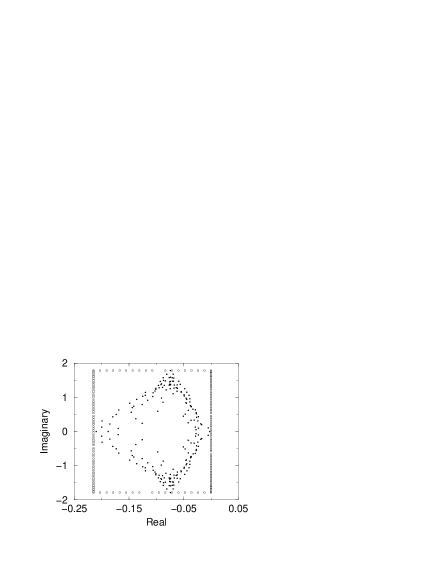
FIG. 3.: Scaled spectrum $L/L^{-}$ of the Liouville superoperator for the model of electron transfer. Approximate eigenvalues obtained in Krylov subspace are plotted as dots. Open squares denote the interpolation points $\lambda_{j}$ for the NP scheme.

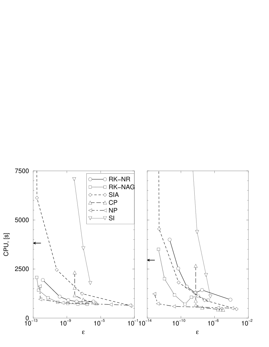
FIG. 4.: Numerical performance of different numerical propagators. Results obtained in the diabatic (adiabatic) representation are shown on the left (right) plot. The arrows represent the numerical performance for the NP propagator with 50 terms and timestep 100 a.u.

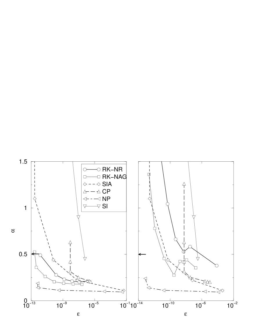
FIG. 5.: Numerical performance of different numerical propagators. The numerical effort $\alpha$ is defined in Section IV. Results obtained in the diabatic (adiabatic) representation are shown on the left (right) panel. The arrows represent the numerical performance for the NP propagator with 50 terms and timestep 100 a.u.