Transport control by coherent zonal flows in the core/edge transitional regime

Abstract

3D Braginskii turbulence simulations show that the energy flux in the core/edge transition region of a tokamak is strongly modulated – locally and on average – by radially propagating, nearly coherent sinusoidal or solitary zonal flows. The flows are geodesic acoustic modes (GAM), which are primarily driven by the Stringer-Winsor term. The flow amplitude together with the average anomalous transport sensitively depend on the GAM frequency and on the magnetic curvature acting on the flows, which could be influenced in a real tokamak, e.g., by shaping the plasma cross section. The local modulation of the turbulence by the flows and the excitation of the flows are due to wave-kinetic effects, which have been studied for the first time in a turbulence simulation.

a Introduction —

It is now commonly believed, that the transport in the tokamak core is controlled by zonal flows [1, 2, 3]. In the plasma edge, the flows were not studied thoroughly yet, but they tend to be weak [4] (although they can possibly completely quench the turbulence [5]). The zonal flows in the core and at the edge were found to be incoherent, random fluctuations [2, 6, 7]. In contrast to this, in the transitional regime between core and edge, strong radially coherent sinusoidal or solitary zonal flows are ubiquitous according to the numerical simulations described below. The zonal flows in the transitional regime are essentially geodesic acoustic modes [8], i.e., the poloidal rotation is coupled to an $(m,n)=(1,0)$ pressure perturbation by the inhomogeneous magnetic field, which results in a restoring force and hence an oscillation. Transcending the present models of the zonal flow generation based purely on Reynolds stress [1], the major part of the flow energy in the transitional regime is apparently generated by the Stringer-Winsor term [9], i.e., the torque on the plasma column caused by the interaction of pressure inhomogeneities with the inhomogeneous magnetic field. An order of magnitude variation of the shear flow level and average transport has been observed upon a sole modification of the curvature terms acting on the flows, at fixed curvature terms acting on the turbulence. The pressure inhomogeneities are driven by anomalous transport modulations, which can be understood by a drift-wave model for the wave-kinetic turbulence response to the flows. Some predictions of the model have been verified subsequently in numerical experiments.

Zonal flows in the transitional regime are GAMs—

The numerical turbulence simulations have been carried out using the three dimensional electrostatic drift Braginskii equations with isothermal electrons, including the ion temperature fluctuations with the associated polarization drift effects, the resistive (non-adiabatic) parallel electron response and the parallel sound waves (a subset of the equations of Ref. [5]). The nondimensional parameters have been varied around a reference parameter set resembling the transitional core/edge regime: $\alpha_{d}=0.6$, $\epsilon_{n}=0.08$, $q=3.1$, $\tau=1$, $\eta_{i}=3$, $\hat{s}=1$. The computational domain is a flux tube winding around the tokamak for three poloidal connection lengths. The radial and poloidal domain width is $50L_{\rm RB}$, with the resistive ballooning scale length, $L_{\rm RB}$. For a definition of these parameters and units see Ref. [5]. The parameters are consistent with the physical parameters $R=3$ m, $a=1.5$ m, $L_{n}=12$ cm, $n=3.5\times 10^{19}$ m^-3, $Z_{\rm eff}=4$, $B_{0}=3.5$ T, and $T=200$ eV, $L_{\rm RB}=3.6$ mm, $\rho_{s}=0.82$ mm. At these parameters the ITG mode turbulence is the dominant cause of the heat flux [4], and the restriction of the domain to a flux tube is justified [7].

Viewed as a function of radius and time, the flux surface averaged poloidal ${\bf E}\times{\bf B}$ flows [fig. 1 (a)] start as an irregular pattern of radially propagating independent wavelets and merge into a radially coherent standing wave later on. The final standing wave pattern consists of GAM oscillations. They can be described by suitable poloidal Fourier components of the vorticity and pressure evolution equations (neglecting the parallel sound wave),

$$\partial_{t}\langle v_{E}\rangle-\langle s_{v}\rangle=-C_{1}\langle p\sin\theta\rangle$$ (1)

$$\partial_{t}\langle p\sin\theta\rangle-\langle s_{p}\sin\theta\rangle=C_{2}\frac{\epsilon_{n}}{3}\frac{3+5\tau}{1+\tau}\langle v_{E}\sin^{2}\theta\rangle,$$ (2)

with $\langle.\rangle$ denoting the flux surface average, the pressure fluctuations $p=n+\frac{\tau}{1+\tau}T_{i}$, the poloidal flow velocity $v_{E}=\partial_{x}\phi$, and the source terms $s_{v}$/$s_{p}$ of flow/pressure due to Reynolds stress/anomalous transport, respectively. For easier reference, the two different curvature terms in the equations have been adorned with the factors $C_{1}$ and $C_{2}$, which are both $1$ in the turbulence equations for a low aspect ratio circular tokamak. The curvature term $C_{1}$ is the Stringer-Winsor term, the term $C_{2}$ represents the up-down asymmetric compression of the plasma due to the poloidal rotation. For all parameters used in the numerical simulations, the zonal flows oscillate in the stationary state with a frequency within $5\%$ of the eigenfrequency of Eqs. (1,2) without source terms and with the approximation $\langle v_{E}\sin^{2}\theta\rangle\approx\langle v_{E}\rangle/2$,

$$\omega=\sqrt{C_{1}C_{2}\frac{\epsilon_{n}}{6}\frac{3+5\tau}{1+\tau}}.$$ (3)

In physical units this is equal to $\sqrt{(6+10\tau)/(3+3\tau)}c_{s}/R\sim c_{s}/R$. Since the parallel sound frequency $c_{s}/(qR)$ is much lower than the GAM frequency, the neglect of the parallel sound wave is justified. The energy balance equation of the GAM oscillations is according to (1,2)

$\displaystyle\partial_{t}\frac{1}{2}\left[\langle v_{E}\rangle^{2}+\frac{C_{1}}{\omega}\langle p\sin\theta\rangle^{2}\right]=$

$$\langle v_{E}\rangle\langle s_{v}\rangle+\frac{C_{1}}{\omega}\langle p\sin\theta\rangle\langle s_{p}\sin\theta\rangle$$ (4)

The average contributions to the GAM energy from the Reynolds stress term $\langle s_{v}\rangle$ and the Stringer-Winsor term $\langle s_{p}\sin\theta\rangle$ have been listed in table I for varying turbulence parameters. In the transitional regime with its strong coherent zonal flows most of the flow energy is generated by the Stringer-Winsor term, while with decreasing temperature toward the very edge the Stringer-Winsor energy input eventually becomes negative indicating a braking force on the flows, while simultaneously we get weak incoherent flows. One is tempted to attribute the decrease of the zonal flows towards the very edge to the Stringer-Winsor term. Indeed, eliminating the flow source term $\langle s_{p}\sin\theta\rangle$ due to the anomalous transport in the numerical simulations leads to relatively strong coherent flows even for parameters in the very edge.

With the natural drive of the GAM being apparently the Stringer-Winsor term, it has been found that altering the amplitude of the curvature terms $C_{1},C_{2}$ acting on the flows but keeping the curvature terms acting on the turbulence modes fixed, changes the flow amplitudes and the anomalous transport by one order of magnitude. Empirically, the flow level rises with increasing $C_{1}$ and decreasing $\omega$. One reason is, that the higher $C_{1}/\omega\sim\sqrt{C_{1}/C_{2}}$ is, the higher is the contribution of the anomalous transport source term $s_{p}$ to the flow energy (4). At constant ratio $C_{1}/\omega$ the flows are still somewhat increasing for decreasing $\omega$. This is understood, since with increasing oscillation period the flows have more time to influence the turbulence resulting in an increased $s_{p}$.

The cause of the pressure perturbations driving the flows are local modulations of the anomalous transport (the usual Stringer spin-up mechanism is ineffective due to the relatively long sound transit time in the considered regime). Plots of the radial pressure transport $\langle v_{r}p\rangle=Q(r,t)$ and its up-down antisymmetric component $\langle v_{r}p\sin\theta\rangle=U(r,t)$ are shown in fig. 1 (b) and (c). (Note that the pressure source term is the divergence of the anomalous pressure flux, i.e., $s_{p}=-\partial_{r}(v_{r}p)$, and $\langle s_{p}\sin\theta\rangle=-\partial_{r}U$.) In the initial phase of flow generation, $U$ develops dipoles around the flows [fig. 1 (d)], in which $U$ has always the same sign as the local shearing rate. These dipolar transport structures generate the pressure up-down asymmetries driving the GAMs. As soon as sufficiently strong flows exist, the anomalous transport $Q$ develops a striking peaking at the radii of positive flow resembling transport fronts propagating with the flow “waves”. In addition to the dipole structures $U$ develops a unipolar part component, whose sign depends on the propagation direction of the corresponding flow. These up-down antisymmetric transport fronts can be viewed as avalanches running outward on the lower half of the torus ($\theta<0$) and inward on the upper half.

The unipolar up-down asymmetries have been found to be responsible for the setup of the flow pattern. If in a numerical experiment the GAMs are initially set to zero outside of one flow peak, the turbulence is still capable of moving this flow into the original direction, until a new standing wave pattern has been formed. The necessary radial GAM energy flow due to the turbulence has been found to be primarily caused by the unipolar up-down asymmetries. Similar events happen, if a numerical simulation is started with a GAM pattern with the wrong wave-length from a simulation run with different GAM parameters. In that case, strong unipolar up-down transport asymmetries develop, which enforce the equilibrium flow propagation velocity, i.e., flow wavelength.

The described peculiar modulation of the transport by the flows is absent for weak diamagnetic drift and vanishing gyro radius, such as in the resistive ballooning regime [4]. Instead, the shear flows simply weaken the turbulence. Apart from this, there is a tendency to flatten pressure gradients, i.e., to eliminate the pressure fluctuations associated with the GAM, resulting in the observed braking force.

The wave-kinetic effects

The dependence of the transport modulation on drift effects and the gyro radius suggests a simplified drift wave model containing only the radial mode coupling due to the polarization drift, eliminating two fluid and curvature effects. Since in the numerical studies the mode wavelengths are not small compared to the zonal flow scales, we refrain from a geometrical optics approach [1] and instead move back to the linearized adiabatic drift wave equation,

$$D_{t}(1-\rho_{s}^{2}{\Delta_{\perp}})\phi+\alpha_{d}\partial_{y}\phi=0,$$ (5)

with $D_{t}=\partial_{t}+v_{E}(x,t)\partial_{y}$. We study the impact of the polarization drift term $-D_{t}\rho_{s}^{2}{\Delta_{\perp}}n$ up to first order in $\rho_{s}^{2}$, without assumptions on the ratio of flow vs. turbulence scales. The 0-th order time evolution (with $y$ in Fourier space) is

$$\phi_{0}(x,t)=\phi_{i}(x)\psi(x,t)$$ (6)

with initial amplitude $\phi_{i}(x)$ and the flow-and-drift induced phase factor

$$\psi(x,t)=\exp\left[-ik_{y}\xi\right],\quad\xi=\int_{0}^{t}\left[v_{E}(x,\tau)+\alpha_{d}\right]d\tau.$$ (7)

Inserting (6) into (5) results in the first order correction $\phi_{1}$ due to $\rho_{s}^{2}$

$\displaystyle\phi_{1}(x,t)\psi^{*}(x,t)=-ik_{y}\alpha_{d}\rho_{s}^{2}\int_{0}^{t}\psi^{*}(x,\tau){\Delta_{\perp}}\left(\phi_{i}\psi(x,\tau)\right)d\tau+$

$$+\rho_{s}^{2}\left[\psi^{*}(x,\tau)\partial_{x}^{2}\left(\phi_{i}\psi(x,\tau)\right)\right]_{\tau=0}^{\tau=t},$$ (8)

in which $[f(\dots,\tau)]_{\tau=0}^{\tau=t}\equiv f(\dots,t)-f(\dots,0)$. From this, the change in turbulence intensity can be computed to first order,

$\displaystyle\delta|\phi|^{2}=2{\rm Re}(\phi_{1}^{*}\phi_{0})=2k_{y}\alpha_{d}\rho_{s}^{2}\int_{0}^{t}\partial_{x}[k_{x}(x,\tau)|\phi_{i}|^{2}]d\tau$

$$-2\rho_{s}^{2}[k_{x}^{2}(t)-k_{x}^{2}(0)]|\phi_{i}|^{2},$$ (9)

with a suitable local $k_{x}(x,\tau)\equiv-k_{y}\xi^{\prime}(x,\tau)+{\rm Im}(\phi_{i}^{\prime}/\phi_{i})$. The term involving the diamagnetic drift velocity $\alpha_{d}$ corresponds to the advection of mode intensity in response to the shearing distortion, while the other term is analogous to the adiabatic compression of a wave field.

If the initial $\phi_{i}$ has no radial structure ($k_{x}=0$) and the shear flows do not change with time, we obtain due to radial mode advection

$$\delta|\phi|^{2}_{\rm advection}=-\rho_{s}^{2}\alpha_{d}|\phi_{i}|^{2}t^{2}k_{y}^{2}v^{\prime\prime}_{e},$$ (10)

which explains the empirical peaking in turbulence intensity at the locations of positive flows. To verify the presence of the advection term, a complementary scenario has been simulated, with the turbulence initially confined to a small region and a constant linear shear flow $v_{E}\propto x$ enforced upon it. This results in a motion of the turbulence maxima towards increasing $v_{E}$, which confirms the presence of the advection term (see fig. 2). In another numerical experiment, a stationary bell shaped flow profile has been superposed on an initially radially homogeneous turbulence field, which has been prepared with the zonal flows switched off. After the turbulence rises transiently at the flow maximum, it drops to a level below the initial one. This corroborates that the turbulence amplification at the flow maxima is not due to an increase of drive at the flow maxima [10], but due to a transient wave-kinetic concentration of fluctuation energy.

The numerically observed radial dipole layers of up-down antisymmetric transport apparently result from the compressional terms in (9) acting on the mode structure enforced by the magnetic shear, namely

$$k_{x}\sim k_{y}\hat{s}\theta.$$ (11)

Hence, with $\hat{s}=1$ a shear flow with positive $v^{\prime}_{e}$ reduces $k_{x}^{2}$ on the upper side of the tokamak ($\theta>0$) increasing the mode amplitude there, while the mode is attenuated for ($\theta<0$). The dependence of the shear flow action on the magnetic shear has been verified in a numerical experiment with $\hat{s}=-1$, in which the modes are amplified for $\theta v^{\prime}_{e}<0$. Moreover, a “swinging through” effect hast been observed, i.e., the turbulence intensity decreases again, when $k_{x}^{2}$ rises after $k_{x}$ has gone through zero.

Last, we consider the unipolar up-down transport asymmetries induced by a propagating positive shear flow (which is accompanied by a general transport peaking due to the advective effect). With $v_{E}(x,t)=V(x-\nu t)$ (propagation velocity $\nu$) we obtain from definition (7) $\xi^{\prime}(x,t)=-\nu^{-1}V(x-\nu t)$, i.e.

$$k_{x}(x,t)^{2}=(k_{x0}-k_{y}\xi^{\prime})^{2}=k_{y}^{2}(\hat{s}\theta+\nu^{-1}V(x-\nu t))^{2}.$$ (12)

A reduction of $k_{x}^{2}$ and corresponding amplification of the turbulence modes via eq. (9) occurs for $\hat{s}\theta\nu V<0$. The sign of this effect of a moving flow has been confirmed numerically for positive and negative shear.

Conclusions —

GAMs, oscillating zonal flows, have been found to be the main mechanism controlling the turbulence level in the transitional core/edge regime. Quasi-stationary zonal flows are unimportant in the simulations, because of the strong restoring force due to the pressure imbalance generated by the magnetic field inhomogeneity, which cannot be short-circuited along the magnetic field lines due to the long parallel sound transit time in the transitional regime. Primarily, the flows are not driven by Reynolds stress but by the pressure asymmetries on a flux surface generated by modulations of the anomalous transport. These modulations in turn are caused by the flows, on one hand by the radial advection of turbulence energy concentrating the turbulence in locations of increased flow in electron diamagnetic direction, and on the other hand by adiabatic compression effects on the wave field which together with the magnetic shear result in up-down asymmetries of the transport. The peculiar nature of the drive mechanism leads to propagating peaked flow structures acompanied by pronounced transport fronts, which sometimes come close to propagating solitons. We have studied for the first time the action of wave-kinetic effects in a numerical simulation. Similar results should be expected for the core, except that the polarization due to the ion larmor radius has to be replaced by the neoclassical polarization due to the banana width [11]. I.e., we expect the wave-kinetic transport modulation in the core to be significantly stronger than in in the edge. GAMs on the other hand are less important in the core due to the shorter parallel connection length ($q\sim 1$).

On one hand, the GAM drive efficency depends on the nature of the turbulence, in that it depends on the presence of finite $\rho_{s}$ effects. Absence of these, such as in the resistive ballooning regime leads to a strong damping of the GAM due to the anomalous diffusion eroding the pressure fluctuations connected with the GAM. However, apart from the turbulence the zonal flow amplitude is influenced strongly by the linear properties of the GAM itself, such as its frequency or the torque excerted on a pressure fluctuation. Manipulation of both of them can lead to a reduction of the transport by up to an order of magnitude. Consequentially, any discussion of the anomalous transport focusing on the influence of the magnetic geometry on the turbulence drive falls short of an essential factor, if the influence of the magnetic geometry on the flows is neglected. Since the GAM properties could be influenced in a real tokamak by, e.g., shaping the plasma column, the coherent flows should be taken into consideration to further reduce the transport in advanced tokamaks. Moreover, the clear signature of the radially coherent flows in the numerical simulations makes them an interesting target of experimental investigation, e.g., by means of microwave reflectometry.

This work has been performed under the auspices of the Center for Interdisciplinary Plasma Science, a joint initiative by the Max-Planck-Institutes for Plasma Physics and for Extraterrestrial Physics.

(a)

(b)

(c)

(d)

FIG. 1.: Time evolution of (a) poloidal ${\bf E}\times{\bf B}$ flow profile, (b) pressure flux profile $\langle v_{r}p\rangle$, (c) up-down asymmetric pressure flux $\langle v_{r}p\sin\theta\rangle$ for the standard parameters; (d) instantaneous profiles at $t=80$ of the flow (above), pressure flux (solid, below), and the up-down asymmetric pressure flux (dashed). Note the dipole layers of up-down asymmetric pressure flux around the flows, e.g., at $x=-7$. The unipolar component of the flux asymmetries can be observed in figure (c): depending on their propagation direction the traces look either bright or dark.

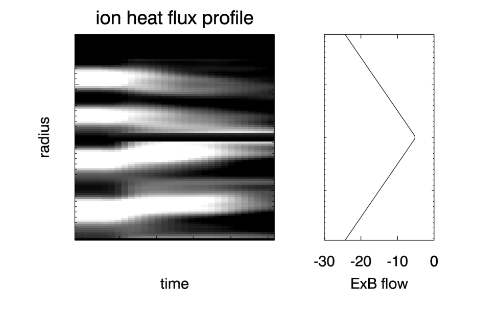
FIG. 2.: Time evolution of heat flux profile demonstrating turbulence movement in responce to a linear shear flow with different sign for the lower and upper half of the plots.

TABLE I.: Mean GAM energy production due to Reynolds stress and Stringer-Winsor effect, flow intensity $\langle v_{E}^{2}\rangle$ and anomalous pressure transport $\langle pv_{r}\rangle$ for varying parameters. The units are the turbulence units described in reference [5]. In these units, the diamagnetic velocity is equal to $\alpha_{d}$. The parameters are consistent with the physical reference parameters given in the text, except for an altered temperature $T_{i}=T_{e}=T$. For $\alpha_{d}=0$ the ions have been assumed cold. In the line marked with an $*$ the Stringer-Winsor drive has been switched off, eliminating its braking force in the ballooning regime.

$\alpha_{d}$	${\eta_{i}}$	$T$ (eV)	$\langle pv_{r}\rangle$	$\langle v_{E}^{2}\rangle$	Reynolds drive	Stringer drive
0	$-$	0	0.27	0.04	$1.4$	$-1.0$
0∗	$-$	0	0.25	0.2	3.3	$-26$
0.2	1	100	0.27	0.03	2.0	$-1.0$
0.2	3	100	0.87	0.23	1.5	3.6
0.6	3	300	0.15	0.9	$-0.1$	10.0
1.1	3	550	0.24	0.9	16.0	33.4

REFERENCES

- [1] P. H. Diamond, M. N. Rosenbluth et al., 17th IAEA Fusion Energy Conference, IAEA-CN-69/TH3/1 (1998)
- [2] T. S. Hahm et al., Phys. Plasmas 6, 922 (1999)
- [3] P. W. Terry, Rev. Mod. Phys. 72, 109 (2000)
- [4] A. Zeiler et al., Phys. Plasmas 5, 2654 (1998)
- [5] B. N. Rogers et al., Phys. Rev. Lett 81, 4396 (1998)
- [6] Z. Lin et al., Phys. Plasmas 7, 1857 (2000)
- [7] K. Hallatschek, Phys. Rev. Lett. 84, 5145 (2000)
- [8] S. V. Novakovskii et al., Phys. Plasmas 4, 4272 (1997)
- [9] A. B. Hassam et al., Phys. Plasmas 1, 337 (1994)
- [10] K. L. Sidikman et al., Phys. Plasmas 1, 1142 (1994)
- [11] M. N. Rosenbluth et al., Phys. Rev. Lett. 80, 724 (1997)
(a)