AUTOMODULATIONS IN KERR-LENS MODELOCKED SOLID-STATE LASERS

Abstract. Nonstationary pulse regimes associated with self modulation of a Kerr-lens modelocked Ti:sapphire laser have been studied experimentally and theoretically. Such laser regimes occur at an intracavity group delay dispersion that is smaller or larger than what is required for stable modelocking and exhibit modulation in pulse amplitude and spectra at frequencies of several hundred kHz. Stabilization of such modulations, leading to an increase in the pulse peak power by a factor of ten, were accomplished by weakly modulating the pump laser with the self-modulation frequency. The main experimental observations can be explained with a round trip model of the fs laser taking into account gain saturation, Kerr lensing, and second- and third-order dispersion.

OCIS: 320.5550, 320.7090, 320.7160, 270.5530

1 Introduction

Nonstationary regimes of ultrashort pulse generation in lasers have gained a great deal of attention in recent years. While the stable operation of femtosecond lasers is usually the preferred mode of operation, nonstationary regimes provide unique opportunities to explore the physical mechanisms leading to the formation and stabilization of ultrashort pulses. The trend to generate ever shorter pulses from laser oscillators makes it desirable to characterize the parameter range of stable operation in detail. This includes the boundaries of such regimes and the processes leading to nonstationary pulse behavior. On the other hand self- or induced modulation of such lasers can increase the peak power at a reduced repetition rate and are thus attractive for pulse amplification or in experiments where oscillators do not provide sufficient pulse energies.

Various self-starting and induced nonstationary pulse modes in femtosecond dye and solid-state lasers have been reported, among them cavity dumping [1], higher-order soliton formation [2, 3], and periodic amplitude modulations [4]. In recent years, several kinds of periodic pulse amplitude modulation have been observed in Ti:sapphire lasers after inserting apertures or adjusting the dispersion [5]. Also cavity dumping [6] and oscillations between transverse modes [7, 8] has successfully been realized in Ti:sapphire lasers. In this paper we describe experiments and theoretical results of automodulations in fs Ti:sapphire lasers that occur with frequencies typical for relaxation oscillations.

There are two major approaches to describe the complexity of femtosecond lasers – the round trip model where the pulse passes through discrete elements and a continuous model where the action of individual laser components is distributed uniformly in an infinitely extended hypothetical material [9]. Both models allow for analytical as well as numerical approaches. The most successful round trip model was developed more than 20 years ago [10] and relied on the expansion of the transfer functions of the individual laser elements. It yielded an analytical sech solution for the pulse envelope. Later, this model was extended to include self-phase modulation and dispersion leading to sech pulse envelopes and tanh phases [11]. In a stationary regime the pulses reproduce after one or several roundtrips and thus exhibit features of solitary waves and solitons.

In fs Ti:sapphire lasers, the major pulse shaping mechanisms are Kerr-lensing, self-phase modulation (SPM) and group delay dispersion (GDD). A large number of theoretical approaches exist to describe various features of such lasers [12 – 16]. The main condition for pulse stability against the build-up of noise (spontaneous emission) is the negative net-gain outside the pulse. While in fs dye lasers this is realized by the interplay of a slow saturable absorber and gain saturation, in KLM solid-state lasers a fast saturable absorber effect due to Kerr-lensing provides the positive gain window. Outside the parameter range for stable pulses, periodic and stochastic pulse modulations have been predicted [17]. Our theoretical approach in this paper is based on a modified roundtrip model [18] and tracks the changes of the amplitude and phase parameters of the pulse from one roundtrip to the next. As we shall see, the inclusion of cavity third-order dispersion is crucial to describe the nonstationary pulse modes.

In the first part of the paper, we describe two different self-modulation modes observed at GDD greater and smaller than what is required for stable modelocking. In the second part we present a theoretical model based on a stability analysis of the Kerr-lens modelocking that explains the main experimental findings.

2 Experimental

A soft-aperture KLM Ti:sapphire laser was set up in the usual 4-mirror configuration with a $3\;\,mm$ thick crystal between two focussing mirrors of $5\;cm$ focal length, two fused silica prisms for dispersion compensation and a $5\%$ outcoupling mirror. It was pumped with $4.5\;W$, all lines of an Ar-ion laser. The two distinctly different regimes of self-modulation A (B) were realized by increasing (decreasing) the insertion of one of the compensating prisms, that is, adding (subtracting) positive GDD starting from stable modelocking.

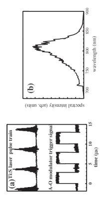
Figure 1: (a) Pulse train from a mode-locked Ti:sapphire laser in a self Q-switched regime A (upper curve) and the acousto-optic driver signal used in the case when the pump laser was modulated. On the time scale shown here there was no observable difference between the Ti:sapphire laser pulse train with the modulated and unmodulated pump laser. (b) Laser spectrum observed during regime A.

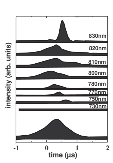
Figure 2: Temporal position of the various spectral components relative to the peak of the Q-switched envelope and the modelocked pulse train (bottom curve).

To obtain regime A, the intracavity prism insertion (glass path) is increased. The spectrum first broadens and blue-shifts until it exhibits a distinct edge at around $730\,\;nm$ and a maximum at $800\;\,nm$. A further increase in the intracavity glass path beyond this point destroys the modelocking. A perturbation of the cavity (e.g. pushing one of the end mirrors or rocking one of the prisms) results in a modulation of the pulse train of the Ti:sapphire laser which can be stabilized by gradually pulling out the prism somewhat. The resulting pulse train and spectrum are shown in Figs.1a (upper curve) and 1b. This modulation is similar to the self Q-switching observed in Ref. [5]. Although the cavity Q is not switched in a strict sense and the modulations rather resemble relaxation oscillations we will keep the term self Q-switching. The peak amplitude under the Q-switch envelope is about ten times higher than the amplitude in the cw modelocked regime. As can be seen from the figure, the self Q-switch period is about $5\;\mu s$ and the width of the Q-switch envelope is about $1\;\mu s$. The Q-switched pulses are separated by pre-lasing regions. The average pulse duration without external pulse compression was measured to be about $130\;fs$ (after $6\;mm$ of SQ1). We compared the second harmonic of the pulse train with the square of the fundamental signal. From that, the pulse duration seemed to be constant over the Q-switched pulse and the prelasing region. Information on the spectral evolution across the Q-switched pulse was gained by recording the output of a fast photodiode placed at the exit slit of a monochromator (bandwidth $15\;nm$). The results shown in Fig. 2 indicate that the spectrum of the pulses under the Q-switched envelope evolves with time on either side of the central wavelength.

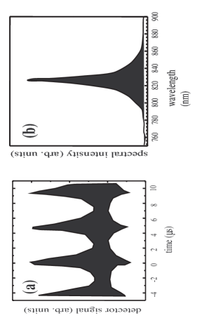
Figure 3: (a) Pulse train and (b) spectrum observed in regime B.

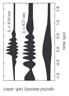
Figure 4: Temporal behavior of spectral components at $810\;nm$ and $827\;nm$ in regime B and the modelocked pulse train (bottom curve).

We observed a second self-modulation mode, B, when the cavity prism was translated so as to decrease the intracavity glass path, that is to increase the negative GDD of the laser cavity. While translating the prism, the spectrum moved towards longer wavelengths and began to narrow until, at a point, the laser jumped into a strongly self-modulated modelocked regime of operation. The modulated pulse train and pulse spectrum are shown in Fig.3a and 3b. Again, no measurable variation of the pulse duration over the modulation period and prelasing region was observed. The pulse duration was about $40\;fs$ (after about $6\;mm$ of SQ1). We also monitored the modulated pulse train through a monochromator. We found strong modulations in the spectral intensity at various wavelengths across the duration of the modulated envelope; some examples are shown in Fig.4. The spectrum (cf. Fig.3b) and the spectral modulations (cf. Fig.4) across the envelope, bear close resemblance to the observation of higher-order solitons reported in Refs. [2] and [3].

Phenomenologically, the existence of regime A can be explained by relaxation oscillations and the interplay of SPM and GDD in the laser. Mode A arises when inserting excess glass into the cavity, that is, introducing positive GDD. According to the soliton model of the laser, a balance of positive chirp due to SPM and negative chirp due to GDD can result in a steady state pulse regime. The prism insertion introduces positive GDD which leaves part of the positive chirp due to SPM uncompensated. SPM is proportional to the product of nonlinear refractive index and pulse intensity and thus dependent on the quotient of pulse energy and duration. Hence, with excess glass, pulses of lower energy but equal pulse duration can still be supported. This comprises the observed prelasing regime. Because of this low intensity lasing, the inversion begins to build up in the gain medium until dumped into the Q-switched pulse. The modulation is driven by relaxation oscillations. In the leading edge of the Q-switched pulse the intensity of the modelocked pulses begins to increase while its duration remains constant. As a result of the higher intensity the SPM begins to generate new spectral components as indicated by the spectral broadening seen later in the Q-switched envelope.

Both modulation regimes A and B were subject to random fluctuations in pulse length, height, and repetition frequency. To stabilize operational mode A, we modulated the pump laser (modulation depth about $5\%$) using an acousto-optic modulator. The modulator was driven by the amplified output of a photodiode that monitored the pulse train of the Ti:sapphire laser. Figure 1a shows the Q-switched pulse train and the trigger signal for the modulator. It was also possible to force modulation with an external oscillator tuned to near the free-running Q-switch frequency of about $200\;kHz$. The more than tenfold increase in the pulse energy in the peak of the Q-switched pulse ( $30\;nJ$) as compared to the ordinary modelocking makes this mode of operation attractive for subsequent high-repetition rate pulse amplifiers and for applications that require a somewhat higher energy than what is available from oscillators.

3 Theory

The aim of this section is to discuss some general aspects of pulse regimes with periodic modulation and then focus on cases that describe our experimental observations, in particular, regime A. To this end we will proceed in two steps, first, second-order group delay dispersion (GDD) is taken into account only, and subsequently, we will add a third-order dispersion term.

Assuming that the change of the pulse envelope during one roundtrip is small, the laser dynamics can be described by a nonlinear equation of the Landau-Ginzburg type [10,19]:

$$\frac{a(k,t)}{k}=\left\{\alpha-l+(1+id)\partial^{2}/\partial t^{2}+(\sigma-i\beta)\left|a\right|^{2}\right\}a(k,t).$$ (1)

Here $a(k,t)$ is the electric field amplitude, $k$ is the round trip number, $t$ is the local time normalized to the inverse gain bandwidth $t_{g}$ which for Ti:sapphire is about $2.5fs$, $\alpha$ is the saturated gain coefficient, $l$ is the linear loss, and $d$ is the GDD coefficient normalized to $t_{g}^{2}$ . The factor before the second derivative, $\left(1+id\right)$ , takes into account GDD and the bandwidth limiting effect of the cavity. For the latter we assume that the bandwidth of the gain medium plays the dominant role. The last summand consists of two parts, a fast absorber (Kerr lensing) term $\sigma\left|a\right|^{2}$ and a self-phase modulation term $-i\beta\left|a\right|^{2}$ . For both terms we assumed saturating behavior according to $\sigma=\sigma_{0}(1-\frac{1}{2}\sigma_{0}\left|a_{0}\right|^{2})$ and $\beta=\beta_{0}(1-\frac{1}{2}\beta_{0}\left|a_{0}\right|^{2})$ , respectively, where $a_{0}$ is the pulse peak amplitude and $\beta_{0}=\frac{2\pi zn_{2}}{\lambda n}$ $=1.7\times 10^{-12\;}cm^{2}/W$ is the unsaturated SPM coefficient for Ti: sapphire crystall. Throughout the paper both $|a_{0}|^{2}$ and $|a|^{2}$ are normalized to $5.9\times 10^{11}\;W/cm^{2}$, then $\beta_{0}$ and $\sigma_{0}$ will be normalized to $1.7\times 10^{-12}\;cm^{2}/W$. The quantity $\sigma_{0}$ plays the role of an inverse saturation intensity of the fast absorber (Kerr-lensing). The larger $\sigma_{0}$ the larger is the amplitude modulation compared to the phase modulation. The quantities $n_{2}$ = $1.3\times 10^{-16}\;cm^{2}/W$ and $n=1.76$ are the nonlinear and linear refractive index, respectively, $z=3\;mm$ is the length of the Kerr medium, and $\lambda=800\;nm$ is the center wavelength. The magnitude of $\sigma_{0}$ can be controlled by the cavity alignment and for typical Kerr-lens modelocked lasers $\sigma_{0}$ is $10^{-10}\;-\;10^{-12}\;cm^{2}/W$ [20]. The saturation of SPM is due for example to the next-higher order term in the expansion for the refractive index, the $n_{4}$ - term. The approximation that the saturation term depends on the peak intensity rather the instantaneous intensity is necessary for solving Eq. (1) analytically.

The gain coefficient, during one roundtrip, changes due to depopulation by the laser pulse, gain relaxation with a characteristic time $T_{31}$ ( $3\;\mu s$ for Ti:sapphire), and the pumping process:

$$\frac{d\alpha}{dt}=\sigma_{14}(\alpha_{m}-\alpha)I_{p}/h\nu_{p}-\sigma_{32}\alpha\left|a\right|^{2}/h\nu-\alpha/T_{31}.$$ (2)

Here $\sigma_{14}$ $=10^{-19}\;cm^{2}$ and $\sigma_{32}$ $=3\times 10^{-19}\;cm^{2}\;$ are the absorption and emission cross-sections of the active medium, respectively, $\alpha_{m}$ is the unsaturated gain coefficient, $\nu_{p}$ and $\nu$ are the pump and laser frequencies, respectively, and $I_{p}$ is the pump intensity. From this equation of the gain evolution one can derive a relation between the gain after the k+1-th roundtrip (left-hand side of the equation, primed quantity) and the k-th roundtrip (right-hand side of equation):

$$\alpha\prime=\alpha\exp(-2\tau\left|a\right|^{2}t_{p}-\frac{T_{cav}}{T_{31}}-U)+\frac{\alpha_{m}U}{(U+T_{cav}/T_{31})}[1-\exp(-\frac{T_{cav}}{T_{31}}-U)],$$ (3)

where $t_{p}$ is the laser pulse duration normalized to $t_{g}$ and $T_{cav}$ ($10\;ns$) is the cavity roundtrip time. The quantity, $\tau^{-1}$ is the gain saturation energy fluency $E_{g}$ ($0.82\;J/cm^{2}$) normalized to $\frac{\lambda nt_{g}}{2\pi zn_{2}}$ ($1.5\times 10^{-3}\;J/cm^{2}$) for which we obtain a value of $555$ that was used in our calculations. $U=\frac{\sigma_{14}T_{cav}}{h\nu_{p}}I_{p}$ is a dimensionless pump parameter, which we chose close to $4\times 10^{-4}$ (for a pump laser spot size of $100\;\mu m$ this corresponds to about $4\;W$ pump power). When analyzing stationary regimes where the pulses reproduce after each roundtrip a steady-state gain coefficient is used that can be obtained by setting $\alpha=\alpha\prime$ in Eq. (3). In the simulation of nonstationary regimes the gain coefficient changes from roundtrip to roundtrip as described by Eq.(3). As is known, see for example [12], Eq. (1) has a quasi-soliton solution of the form

$$a(t)=a_{0}\exp(i\phi)/\cosh^{1+i\psi}(t/t_{p}),$$ (4)

where $\psi$ is the chirp term, and $\phi$ is the constant phase accumulated in one cavity roundtrip. To investigate the pulse stability we used a so-called aberrationless approximation [21], which allows one to investigate the dependence of the pulse parameters on the roundtrip number $k$. After substituting the ansatz (4) into Eq. (1) and expanding of obtained equation in series of $t$ up to third order, we obtain three ordinary differential equations as coefficients of expansion. The solution of the obtained system by the forward Euler method relates the unknown pulse duration $t_{p}$, chirp parameter $\psi$, and peak amplitude $a_{0}$ after the $k+1$-th roundtrip (left-hand side of the equation, primed quantities) to the pulse parameters after the $k$-th transit (right hand side of the equations):

$$t_{p}\prime=t_{p}+\frac{4-7d\psi-3\psi^{2}+(\phi\psi-2\sigma a_{0}^{2}-\psi\beta a_{0}^{2})t_{p}^{2}}{2t_{p}^{2}},$$ (5)

$$\psi\prime=(1-2\sigma a_{0}^{2})\psi+(\phi-\beta a_{0}^{2})\psi^{2}+\phi-3\beta a_{0}^{2}-\frac{5d+3\psi+5d\psi^{2}+3\psi^{3}}{t_{p}^{2}},$$ (6)

$$a_{0}\prime=a_{0}[1+\frac{d\psi-1+(\alpha-l-\sigma a_{0}^{2})t_{p}^{2}}{t_{p}^{2}}].$$ (7)

A fourth equation yields the phase delay,

$$\phi=\beta a_{0}^{2}+\frac{d+\psi}{t_{p}^{2}}.$$ (8)

Equations (5-8) describe a stationary pulse regime if the complex pulse envelope reproduces itself after one cavity roundtrip, that is, the pulse parameters to the left and the right of the equal sign are identical. Within a certain range of laser parameters such a stationary regime usually develops after a few thousand roundtrips and the stationary pulse parameters can be obtained by solving the system of algebraic equations. In an unstable or periodically modulated pulse regime, the evolution of the pulses can be followed by calculating the new pulse parameters after one additional roundtrip and using these results in the right-hand side of Eqs. (5-8), i.e., as input for the next roundtrip.

We will first study the behavior of the laser when the SPM parameter $\beta_{0}$ and the self-amplitude parameter $\sigma_{0}$ are varied. Physically this can be accomplished by changing the focusing into the crystal and by changing the cavity alignment or by inserting intracavity apertures, respectively.

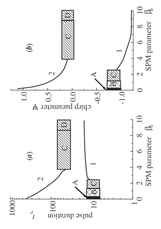
Figure 5: Steady-state pulse duration (a) and chirp (b) versus the normalized SPM coefficient $\beta_{0}$ for a normalized GDD coefficient of $d=0$ (curve 1) and $d=-10$ (curve 2). The other laser parameters are $\sigma_{0}$ $=1$, $l=0.05$, $\alpha_{m}$ $=0.5$, $U=4\times 10^{-4}$, $z=0.3\;cm$, $\lambda=800\;nm$, and $T_{cav}=10\;ns$. The hatched regions describe various nonstationary pulse regimes, see text.

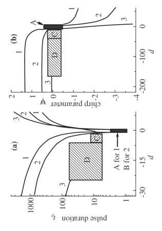
Figure 6: Steady-state pulse duration (a) and chirp (b) versus the normalized GDD coefficient $d$ for $\beta_{0}=1$ and $\sigma_{0}=10$ (curve 1), $\sigma_{0}=1$ (curve 2), $\sigma_{0}=0.1$ (curve 3). The other parameters are the same as in Fig. 5.

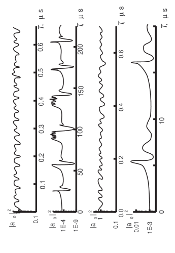
Figure 7: The normalized pulse intensity $|a_{0}|^{2}$ (log scale) versus global time $T$. The laser parameters for the different curves are chosen as follows. curve a: $U=4\times 10^{-4}$, $\beta_{0}=0$, $d=0$, $\sigma_{0}$ $=1$ curve b: $U=5\times 10^{-4}$, $\beta_{0}$ $=0$, $d=-10$, $\sigma_{0}$ $=1$ curve c: $U=4\times 10^{-4}$, $\beta_{0}$ $=1$, $d=0$, $\sigma_{0}$ $=1$ curve d: $U=6\times 10^{-4}$, $\beta_{0}$ $=1$, $d=-20$, $\sigma_{0}$ $=0.1$

Figures 5, 6, and 7 summarize our evaluation of the mode-locking based on Eqs. (5-8). Figures 5 and 6 show pulse duration and chirp as a function of the SPM parameter $\beta_{0}$ and the GDD parameter $d$, respectively. The solid curves describe steady-state regimes where the pulse parameters reproduce themselves after one roundtrip while the rectangles indicate various unstable or periodic pulse modes. Note that these areas refer to a certain part of a curve rather than to a two-dimensional parameter range. In region A regular (periodic) oscillations of the pulse parameters occur while in region B these oscillations are irregular. Region C denotes the parameter range where there is no solution to Eq. (1) in the form of ansatz (4). Region D describes oscillations that have a quasi-regular character. Figure 7 depicts the normalized pulse intensity versus the global time $T=T_{cav}k$ .

Curve 1 of Fig. 5 describes the (hypothetical) situation of zero GDD. For small SPM, $\beta_{0}$ $<$ $0.016$ (region A), the pulse regime is unstable. A closer inspection, see Fig. 7a, reveals regular oscillations of the pulse amplitude in this parameter range. The Fourier spectrum of these oscillations shows seven peaks that broaden rapidly if the pump power is increased. The resulting broad frequency spectrum indicates a chaotic behavior of the pulse parameters. An example of the strong dependence of the amplitude modulation on the pump power is illustrated in Fig. 7, curve a and b. A further increase of the SPM, $0.016<$ $\beta_{0}$ $<$ $1.3$ (region B), leads to irregular oscillations of the pulse parameters, as can be seen in Fig. 7c. Even larger SPM, $\beta_{0}$ $>$ $2.6$, results in stable pulses.

Curve 2 in Fig. 5 is in the presence of GDD. A comparison with curve 1 shows, that GDD stabilizes the pulse generation in the region of small $\beta_{0}$, $\beta_{0}$ $<$ $3.9$, however at substantially longer pulses. We explain the stabilization to be due mainly to a smaller effect of nonlinearities as a result of the longer pulse duration and the subsequently lower intensities. In all cases depicted in Figs. 5 and 6, approaching regions of instability means increasing the pulse energy. This leads to stronger gain saturation which makes the onset of relaxation-oscillation driven instabilities more likely.

Figure 6 depicts pulse duration and chirp as a function of the GDD parameter $d$ for a constant SPM parameter $\beta_{0}=1$ and different $\sigma_{0}$ , that is, different magnitude of the amplitude modulation term. Stable pulses over a broad range of the GDD can be expected for larger values of $\sigma_{0}$ (curves 1 and 2). There is no stable regime near zero GDD (solid rectangle). For small values of $\sigma_{0}$ (curve 3) there is a broad range of unstable pulse behavior (area D). Stable pulses occur at large negative GDD and around zero and positive GDD. Except for a region near zero GDD, a larger $\sigma_{0}$ results in longer pulses.

In summary, two distinctly different stable pulse modes exist. One where the effective phase nonlinearity $\beta_{0}$ is large (cf. Fig. 5, curve 1) or where long pulses and therefore low intensities (cf. Fig. 5, curve 2) result in strongly chirped output pulses (Fig. 5b). In these regimes any pulse shortening due to the fast absorber action and spectral broadening due to SPM is counteracted by the bandwidth-limiting element. The second mode shows the features of solitary pulse shaping, that is the interplay of GDD and SPM nonlinearity results in a quasi-Schrödinger soliton pulse with small chirp (cf. Fig. 6b, curve 3 to the left of region D). The pulse area agrees with what is predicted from the nonlinear Schrödinger equation for a fundamental soliton.

At small $\sigma_{0}$ (curve 3, Fig. 6), decreasing the amount of negative GDD from the stable pulse regime results in periodic oscillations of the pulse intensity (region D). This behavior describes our experimental observations, cf. Figs. 1 and 2. The calculated temporal evolution of the pulse amplitude is detailed in Fig. 7d. The Q-switch period is close to the gain relaxation time $T_{31}$, a fact that supports the notion that this behavior is driven by relaxation oscillations.

The experimental observations were made near zero GDD where higher-order dispersion effects are more likely to play a role. Therefore, in the next step, we included a third-order dispersion term in our model, i.e., we added a term $d_{3}\partial^{3}/\partial t^{3}$ to Eq. (1). Here $d_{3}$ is a dimensionless third-order dispersion coefficient, which is normalized $t_{g}^{3}$. To solve the resulting differential equation we now make the ansatz

$$a(k,t)=a_{0}sech^{1+i\psi}[(t-\vartheta k)/t_{p}]\/\,\,\/e^{i[\phi k+\omega(t-\vartheta k)]},$$ (9)

where $\vartheta$ is the pulse delay after one full round trip with respect to the local time frame, and $\omega$ is the frequency detuning from the center frequency of the bandwidth-limiting element [22]. These two additional parameters become necessary in order to describe the effect of third-order dispersion. After inserting the ansatz (9) into the modified laser equation (1), we now obtain six iterative relations for the pulse parameters. The first three equations are comprised of Eqs. (5-7) supplemented by the additional terms

$$-\omega(21d_{3}\psi+\vartheta\psi t_{p}^{2})-d\psi\omega^{2}t_{p}^{2}-d_{3}\omega^{3}\psi t_{p}^{2},$$

$$\omega(3\vartheta+\theta\psi^{2}-[25+9\psi^{2}]d_{3}/t_{p}^{2})-\omega^{2}(6d-5\psi$$

$$-d\psi^{2}+\phi t_{p}^{2}-\sigma a_{0}^{2}t_{p}^{2})-\omega^{3}(10d_{3}-d_{3}\psi^{2}+\vartheta t_{p}^{2})-$$

$$d\omega^{4}t_{p}^{2}-d_{3}\omega^{5}t_{p}^{2},$$

$$3d_{3}\omega\psi-\omega^{2}t_{p}^{2},$$

respectively. To the expression for the phase delay [Eq.(8)] the term $\omega(3d_{3}\omega/t_{p}^{2}-\vartheta)+d\omega^{2}+d_{3}\omega^{3}$ has to be added. The two additional equations for the pulse delay per roundtrip $\vartheta$ and frequency detuning $\omega$ are

$$\vartheta=\frac{\omega(2-4d\psi+2d^{2}\psi^{2})+\omega^{2}d_{3}(9d\psi^{2}-\psi)+9\omega^{3}d_{3}^{2}\psi^{2}-8d_{3}\psi(\alpha-l+\sigma a_{0}^{2})}{-\psi+d\psi^{2}+3d_{3}\omega\psi^{2}},$$ (10)

and

$$\omega\prime=\omega+\frac{8d_{3}\psi-t_{p}^{2}[2\omega+\vartheta\psi-2d\omega\psi-3d_{3}\psi\omega^{2}]}{t_{p}^{4}},$$ (11)

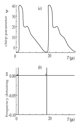
Figure 8: Pulse chirp $\psi$ (a) and normalized frequency shift $\omega$ (b) versus global time $T$ for the laser parameters used in Fig. 7, curve D, and normalized parameter $d_{3}=-30$.

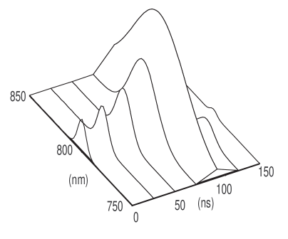
Figure 9: Calculated pulse spectrum at different times near the peak of the Q-switched pulse for the parameters of Fig. 8.

respectively. As is obvious from Eqs. (10) and (11), a nonzero third-order dispersion term gives rise to a pulse group delay (with respect to the local time) and a detuning of the carrier frequency from the center of the bandwidth-limiting element. Figures 8a and 8b show the chirp evolution and the frequency shift plotted for the same parameters as used in Fig. 7d and with $d_{3}=-30$. In Fig.7d a stable pulse operation is periodically disturbed by an increase in the pulse amplitude. Figure 8 is a zoomed-in snapshot describing the chirp and frequency shift during these bursts. Figure 9 shows in detail the evolution of the pulse spectrum near the peak of the Q-switched pulse envelope. The calculated time dependent spectral features are in qualitative agreement with the experimental observations shown in Fig. 2.

4 Conclusions

Kerr-lens modelocked Ti:sapphire lasers can be operated in regimes where periodic oscillations of the pulse amplitude on a time scale of several hundred kHz exist. Two such regimes were observed at intracavity group delay dispersion larger or smaller than what is required for stable modelocking. Stabilization of the pulse amplitude modulation can be accomplished by weakly modulating the pump laser with a signal derived from the modulated Ti:sapphire pulse train. The nature of the self-modulation is similar to relaxation oscillations well known in solid state lasers. A theoretical model of the femtosecond laser that takes into account gain saturation, dispersion, self-phase modulation, and Kerr-lensing explains the trigger of the self-modulations by the interplay of nonlinear self-phase modulation and dispersion. In particular, the strong variation of the pulse spectrum observed during the oscillation spikes can be explained by the theory when third-order dispersion is included. Depending on the relative contribution of SPM and GDD two different pulse stabilization mechanisms exist – the interaction of strongly chirped pulses with the bandwidth-limiting element, and the Schrödinger-soliton stabilization mechanism for nearly chirp-free pulses. The basic calculations in framework of the computer algebra system Maple are available on the site http://www.geocities.com/optomaplev.

5 Acknowledgements

This work was supported in part by the W. M. Keck Foundation and the National Science Foundation (PHY-9601890). V.L.K, I.G.P, and D.O.K acknowledge financial support from the Belorussian Foundation for Basic Research (F97-256).

6 References:

[1] E. W. Castner, J. J. Korpershoek and D. A. Wiersma , “Experimental and theoretical analysis of linear femtosecond dye lasers”, Opt. Comm. 78, 90 (1990).

[2] T.Tsang, “ Observation of high-order solitons from a modelocked Ti:sapphire laser”, Opt. Lett. 18, 293 (1993).

[3] F. W. Wise, I. A. Walmsley and C. L. Tang, “Simultaneous formation of solitons and dispersive waves in a femtosecond dye ring laser”, Opt. Lett. 13, 129 (1988).

[4] V. Petrov, W. Rudolph, U. Stamm and B. Wilhelmi, “Limits of ultrashort pulse generation in cw modelocked dye lasers”, Phys. Rev. A 40, 1474 (1989).

[5] Q. R. Xing, W. L. Zhang and K. M. Yoo, “Self-Q-switched self-modelocked Ti:sapphire laser”, Opt. Comm. 119, 113 (1995).

[6] A. Baltuska, Z. Wei, M. S. Pshenichnikov, D. A. Wiersma and R. Szipöcs, “Optical pulse compression to 5 fs at 1 MHz repetition rate”, App. Phys. B 65, 175 (1997).

[7] D. Cote, H. M. van Driel, “Period doubling of a femtosecond Ti: sapphire laser by total mode locking”, Opt. Lett. 23, 715 (1998).

[8] Bolton S. R, Jenks R. A., Elkinton C. N., Sucha G., “Pulse-resolved measurements of subharmonic oscillations in a Kerr-lens mode-locked Ti: sapphire laser”, J. Opt. Soc. Am. B 16, 339 (1999).

[9] J. C. Diels and W. Rudolph, Ultrashort Laser Pulse Phenomena, Academic Press, San Diego (1996).

[10] H. Haus, “Theory of mode locking with a fast saturable absorber”, J. Appl. Phys. 46, 3049 (1975).

[11] D. Kühlke, W. Rudolph and B. Wilhelmi, IEEE J. Quantum Electron. 19, 526 (1983).

[12] H. A. Haus, J. G. Fujimoto, E. P. Ippen, “Analytic theory of additive pulse and Kerr lens mode locking”, IEEE J. Quant. Electr., QE-28, 2086 (1992).

[13] T. Brabec, Ch. Spielmann, P. F. Curley, and F. Krausz, “Kerr lens mode locking”, Opt. Lett. 17, 1292 (1992).

[14] J. L. A. Chilla, and O. E. Martinez, “Spatio-temporal analysis of the self-mode-locked Ti:sapphire laser”, J. Opt. Soc. Am. B 10, 638 (1993).

[15] V. Magni, G. Cerullo, S de Silvestri and A. Monguzzi, “Astigmatism in Gaussian-beam self-focusing and in resonators for Kerr-lens mode locking”, J. Opt. Soc. Am. B 12, 476 (1995).

[16] V. P. Kalosha, M. Müller, J. Herrmann, and G. Gatz “Spatiopemporal model of femtosecond pulse generation in Kerr-lens mode-locked solid-state lasers”, J. Opt. Soc. Am. B 15, 535 (1998).

[17] V. L. Kalashnikov, I. G. Poloyko, V. P. Mikhailov, D. von der Linde, “Regular, quasi-periodic and chaotic behavior in cw solid-state Kerr-lens mode-locked lasers”, J. Opt. Soc. Am. B 14, 2691 (1997).

[18] V. L. Kalashnikov, V. P. Kalosha, I. G. Poloyko, V. P. Mikhailov, M. I. Demchuk, I. G. Koltchanov, H. J. Eichler, “Frequency-shift locking of continuouse-wave solid-state lasers”, J. Opt. Soc. Am. B 12, 2078 (1995).

[19] F. X. Kärtner, I. D. Jung, and U. Keller, “Soliton mode locking with saturable absorbers : theory and experiments”, IEEE J. Selected Topics in Quant. Electr., 2, 540 (1996).

[20] J. Herrmann, “Theory of Kerr-lens mode locking: role of self-focusing and radially varying gain”, J. Opt. Soc. Am. B 11, 498 (1994).

[21] A. M. Sergeev, E. V. Vanin, F. W. Wise, “Stability of passively modelocked lasers with fast saturable absorbers”, Opt. Commun., 140, 61 (1997).

[22] V. L. Kalashnikov, V. P. Kalosha, I. G. Poloyko, V. P. Mikhailov, “New principle of formation of ultrashort pulses in solid-state lasers with self-phase-modulation and gain saturation”, Quantum Electr., 26, 236 (1996).