A Generalization of the Maximum Noise Fraction Transform

Abstract

A generalization of the maximum noise fraction (MNF) transform is proposed. Powers of each band are included as new bands before the MNF transform is performed. The generalized MNF (GMNF) is shown to perform better than the MNF on a time dependent airborne electromagnetic (AEM) data filtering problem.

I Introduction

The maximum noise fraction (MNF) transform was introduced by Green et al. [1]. It is similar to the principle component transform [2] in that it consists of a linear transform of the original data. However, the MNF transform orders the bands in terms of noise fraction.

One application of the MNF transform is noise filtering of multivariate data [1]. The data is MNF transformed, the high noise fraction bands are filtered and then the reverse transform is performed.

We show an example where the MNF noise removal adds artificial features due to the nonlinear relationship between the different variables of the data. A polynomial generalization of the MNF is introduced which removes this problem.

In Section II we summarize the MNF procedure. The problem data set is introduced in Section III and the MNF is applied to it. In Section IV, the generalized MNF transform is explained and applied. The conclusions are given in Section V.

II The Maximum Noise Fraction (MNF) Transform

In this section we define the MNF transform and list some of its properties. For further details the reader is referred to Green et al. [1] and Switzer and Green [3]. A good review is also given by Nielsen [4]. A reformulation of the MNF transform as the noise-adjusted principle component (NAPC) transform was given by Lee et al. [5]. An efficient method of computing the MNF transform is given by Roger [6].

Let

$$Z_{i}(x),\quad i=1,\ldots,p$$

be a multivariate data set with $p$ bands and with $x$ giving the position of the sample. The means of $Z_{i}(x)$ are assumed to be zero. The data can always be made to approximately satisfy this assumption by subtracting the sample means. An additive noise model is assumed:

$$Z(x)=S(x)+N(x)$$

where $Z^{T}(x)=\{Z_{1}(x),\ldots,Z_{p}(x)\}$ is the corrupted signal and $S(x)$ and $N(x)$ are the uncorrelated signal and noise components of $Z(x)$. The covariance matrices are related by:

$$\mbox{Cov}\{Z(x)\}=\Sigma=\Sigma_{S}+\Sigma_{N}$$

where $\Sigma_{N}$ and $\Sigma_{S}$ are the noise and signal covariance matrices.

The noise fraction of the $i$th band is defined as

$$\mbox{Var}\{N_{i}(x)\}/\mbox{Var}\{Z_{i}(x)\}.$$

The maximum noise fraction transform (MNF) results in a new $p$ band uncorrelated data set which is a linear transform of the original data:

$$Y(x)=A^{T}Z(x).$$

The linear transform coefficients, $A$, are found by solving the eigenvalue equation:

$$A\Sigma_{N}\Sigma^{-1}=\Lambda A$$ (1)

where $\Lambda$ is a diagonal matrix of the eigenvalues, $\lambda_{i}$. The noise fraction in $Y_{i}(x)$ is given by $\lambda_{i}$. By convention the $\lambda_{i}$ are ordered so that $\lambda_{1}\geq\lambda_{2}\geq\ldots\geq\lambda_{p}$. Thus the MNF transformed data will be arranged in bands of decreasing noise fraction. The proportion of the noise variance described by the first $r$ MNF bands is given by

$$\frac{\sum_{i=1}^{r}\lambda_{i}}{\sum_{i=1}^{p}\lambda_{i}}.$$

The eigenvectors are normed so that $A^{T}\Sigma A$ is equal to an identity matrix.

The advantages of the MNF transform over the PC transform are that it is invariant to linear transforms on the data and the MNF transformed bands are ordered by noise fraction.

The high noise fraction bands can be filtered and then the transform reversed. This can lead to an improvement in the filtering results because the high noise fraction bands should contain less signal that might be distorted by the filtering. Examples of this approach have been given by Green et al. [1], Nielsen and Larsen [7] and Lee et al. [5].

An extreme version of MNF filtering is based on excluding the effects of the first $r$ components. That is $r$ is chosen so as to include only bands with high enough noise ratios. This can be achieved by:

$$Z^{*}(x)=(A^{-1})^{T}RA^{T}Z(x)$$ (2)

where $Z^{*}(x)$ is the filtered data and $R$ is an identity matrix with the first $r$ diagonal elements set to zero. Thus eliminating the effect of one or more of the MNF bands produces a filtered data set which is a linear transform of the original data. This MNF based filter uses interband correlation to remove noise.

In order to use Equation (1) to compute $A$, $\Sigma_{N}$ has to be known. Nielsen and Larsen [7] have given four different ways of estimating $N(x)$. They all rely on the data being spatially correlated. A simple method for computing $N(x)$ is by

$$N(x)=Z(x)-Z(x+\delta)$$ (3)

where $\delta$ is an appropriately determined step length. We are effectively assuming

$$S(x)=S(x+\delta).$$

To the extent that this is not true, the estimate of $N(x)$ is in error.

When this method of noise estimation is used, the MNF transform is equivalent to the min / max autocorrelation factor transform [3].

III Airborne Electromagnetic Data

We test the MNF filtering methodology on a flight line produced by SPECTREM’s time dependent airborne electromagnetic (AEM) system. Background information on this AEM system has been explained by Leggatt [8]. A multiband image can be formed by consecutive flight lines but usually each flight line is examined separately.

Fig. 1 shows a flight line of data, consisting of the seven windowed AEM X band spectra. All seven bands are displayed stacked above each other.

Figure 1: Unfiltered AEM data. Bands 1 to 7 are shown. The band number of each spectrum is labelled to the left of the spectrum. The dotted line of each spectrum marks the zero amplitude for that spectrum.

The amplitude of a band at a particular point is proportional to the vertical distance of the spectrum from its corresponding zero amplitude reference (dotted) line. Neighbouring points along a line are responses from neighbouring points on the ground. The higher band numbers are associated with greater underground depths.

Ore bodies are often associated with small features in the higher bands. Analysis can be made easier by filtering the spectra. Because this data set has substantial interband correlation, the MNF filtering methodology can be used.

Fig. 2 (b) shows the MNF filtering of the spectra in Fig. 1. Only the last three bands (i.e. 5, 6 and 7) and a portion of the flight line are shown.

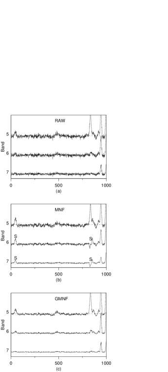
Figure 2: A comparison of the MNF and GMNF filtering methods. Only a portion of the flight line for bands 5, 6 and 7 is shown for each figure. The sample number is displayed on the horizontal axis of each subplot. (a) Unfiltered AEM data. (b) MNF filtered AEM data. The ‘S’ symbols mark parts of the data where spurious features have been introduced by the MNF filtering. (c) GMNF filtered AEM data.

The noise was estimated by taking the difference in neighboring pixels, as in Equation (3). The data were filtered by excluding the first two MNF bands which accounted for approximately 86% of the noise fraction. Although the noise has been reduced, spurious features have been added, indicated by ‘S’. Excluding only the last MNF component does not significantly reduce the magnitude of the spurious features and does almost no noise reduction.

As seen in Equation (2), the MNF filtered data is composed from a linear function of the original data. Fig. 3 shows a plot of $Z_{1}(x)$ against $R_{Z_{1}}(x)$, where $R_{Z_{1}}(x)$ is the difference between $Z_{1}(x)$ and a least squares regression of $Z_{1}(x)$ based on all the other bands.

Figure 3: A plot of the residual of a linear regression of band 1 based on bands 2 to 7, versus band 1 values.

The clear pattern of the residuals plotted in Fig. 3 is evidence that the relationship between $Z_{1}(x)$ and the other bands is not linear. Similar patterned residuals were found for residual plots based on the other bands. In the next section we show how the linear assumption can be relaxed.

IV The Generalized Maximum Noise Fraction Transform

From the discussion in the previous section it appears that using a linear filter is too restrictive for this data set. Gnanadesikan [9] proposed a generalization of the principle component transform. Powers of the original bands were appended to the data set as new bands. For example, $p$ new bands can be created by appending the square of each band to the original data set. Thus each generalized principle component would be a polynomial, as opposed to linear, function of all the bands in the original data set.

The same procedure can be applied to generalize the MNF transform. More formally, a new data set, $Z^{\prime}(x)$, can be created by appending up to $q$ powers of the original data set:

$$Z^{\prime}(x) = \{Z_{1}(x),Z_{2}(x),\ldots,Z_{p}(x),Z_{1}^{2}(x),Z_{2}^{2}(x),\ldots,Z_{p}^{2}(x),\ldots,$$

$$\mbox{}Z_{1}(x)^{q},\ldots,Z_{p}^{q}(x)\}.$$

We are assuming that the $Z_{i}(x)$ have zero means. Cross terms, such as $Z_{1}(x)Z_{2}(x)$ can also be appended. The rest of the methodology remains unchanged.

From Equation (2), each band of the generalized MNF (GMNF) filtered data can be seen to be,

$$Z^{*}_{i}(x)=\sum_{j=1}^{p}\sum_{k=1}^{q}F_{i,j+(k-1)p}Z_{j}^{k}(x)$$

where $F_{i,j+(k-1)p}$ is the element in row $i$ and column $j+(k-1)p$ of the filter matrix:

$$F=(A^{-1})^{T}RA^{T}$$

Thus the GMNF transform leads to a polynomial filter.

To apply the GMNF filter to the data in Fig. 1, the GMNF transform was applied with powers of up to order 6 for each band appended to the original data. Cross terms were found to make little difference to the result and so were not included. The first 15 of the 42 GMNF components, contributing approximately 80% of the noise fraction, were eliminated.

Fig. 2(c) shows the GMNF filtered AEM data. A comparison with the MNF filtered data (Fig. 2(b)) shows that for GMNF filtered data , the noise reduction is greater and spurious features are much less evident.

V Conclusion

We have proposed a generalized maximum noise fraction transform (GMNF) that is a polynomial as opposed to linear transform. The GMNF was applied to filtering a test AEM data set. It was found to remove more noise while adding less artificial features than the MNF based filter.

Implementing the GMNF is a simple extension of the MNF implementation. Software written for the MNF transform can be be used for the GMNF transform without any modification.

References

- [1] A. A. Green, M. Berman, P. Switzer, and M. D. Craig, “A transformation for ordering multispectral data in terms of image quality with implications for noise removal,” IEEE Transactions on Geoscience and Remote Sensing, vol. 26, no. 1, pp. 65–74, 1988.
- [2] Rafael C. Gonzalez and Richard E. Woods, Digital Image Processing, Addison-Wesley publishing company, 1992.
- [3] P. Switzer and A. Green, “Min/max autocorrelation factors for multivariate spatial imagery,” Tech. Rep. 6, Department of Statistics, Standford University, 1984.
- [4] Alan Aasbjerg Nielsen, Analysis of Regularly and Irregularly Sampled Spatial, Multivariate, and Multi-temporal Data, Ph.D. thesis, Institute of Mathematical Modelling. University of Denmark, 1994.
- [5] J. B. Lee, A. S. Woodyatt, and M. Berman, “Enhancement of high spectral resolution remote-sensing data by a noise-adjusted principal components transform,” IEEE Transactions on Geoscience and Remote Sensing, vol. 28, no. 3, pp. 295–304, 1990.
- [6] R. E. Roger, “A faster way to compute the noise-adjusted principal components transform matrix.,” IEEE Transactions on Geoscience and Remote Sensing, vol. 32, no. 6, 1994.
- [7] Alan Aasbjerg Nielsen and R. Larsen, “Restoration of GERIS data using the maximum noise fractions transform,” in Proceedings form the First International Airborne Remote Sensing Conference and Exhibition, Volume II, Strasbourg, France, 1994, pp. 557–568.
- [8] Peter Bethune Leggatt, Some Algorithms and Code for the Computation of the Step Response Secondary EMF Signal for the SPECTREM AEM System, Ph.D. thesis, University of the Witwatersrand, Johannesburg, South Africa, 1996.
- [9] R. Gnanadesikan and M. B. Wilk, “Data analytic methods in multivariate statistical analysis,” in Multivariate Analysis II, P. R. Krishnaiah, Ed. 1969, pp. 593–638, Academic Press. New York, U. S. A.