Transitions induced by the discreteness of molecules in a small autocatalytic system

Abstract

Autocatalytic reaction system with a small number of molecules is studied numerically by stochastic particle simulations. A novel state due to fluctuation and discreteness in molecular numbers is found, characterized as extinction of molecule species alternately in the autocatalytic reaction loop. Phase transition to this state with the change of the system size and flow is studied, while a single-molecule switch of the molecule distributions is reported. Relevance of the results to intracellular processes are briefly discussed.

PACS numbers: 87.16.-b, 05.40.-a

Cellular activities are supported by biochemical reactions in a cell. To study biochemical dynamic processes, rate equation for chemical reactions are often adopted for the change of chemical concentrations. However, the number of molecules in a cell is often rather small [1], and it is not trivial if the rate equation approach based on the continuum limit is always justified. For example, in cell transduction even a single molecule can switch the biochemical state of a cell [2]. In our visual system, a single photon in retina is amplified to a macroscopic level [3].

Of course, fluctuations due to a finite number of molecules is discussed by stochastic differential equation (SDE) adding a noise term to the rate equation for the concentration [4, 5]. This noise term sometimes introduces a non-trivial effect, as discussed as noise-induced phase transition [6], noise-induced order [7], stochastic resonance [8], and so forth. Still, these studies assume that the average dynamics are governed by the continuum limit, and the noise term is added as a perturbation to it.

In a cell, often the number of some molecules is very small, and may go down very close to or equal to 0. In this case, the change of the number between zero and nonzero, together with the fluctuations may cause a drastic effect that cannot be treated by SDE. Possibility of some order different from macroscopic dissipative structure is also discussed by Mikhailov and Hess [9, 10] (see also Ref. [11]). Here we present a simple example with a phenomenon intrinsic to a system with a small number of molecules where both the fluctuations and digitality(‘0/1’) are essential.

In nonlinear dynamics, drastic effect of a single molecule may be expected if a small change is amplified. Indeed, autocatalytic reaction widely seen in a cell, provides a candidate for such amplification [12, 13]. Here we consider the simplest example of autocatalytic reaction networks (loops) with a non-trivial finite-number effect. With a cell in mind, we consider reaction of molecules in a container, contacted with a reservoir of molecules. The autocatalytic reaction loop is $X_{i}+X_{i+1}\rightarrow 2X_{i+1};i=1,\cdots,k;X_{k+1}\equiv X_{1}\\$ within a container. Through the contact with a reservoir, each molecule $X_{i}$ diffuses in and out.

Assuming that the chemicals are well stirred in the container, our system is characterized by the number of molecules $N_{i}$ of the chemical $X_{i}$ in the container with the volume $V$ [14]. In the continuum limit with a large number of molecules, the evolution of concentrations $x_{i}\equiv N_{i}/V$ is represented by

$$dx_{i}/dt=r_{i}x_{i-1}x_{i}-r_{i+1}x_{i}x_{i+1}+D_{i}(s_{i}-x_{i})$$ (1)

where $r_{i}$ is the reaction rate, $D_{i}$ is the diffusion rate across the surface of the container, and $s_{i}$ is the concentration of the molecule in the reservoir.

For simplicity, we consider the case $r_{i}=r$, $D_{i}=D$, and $s_{i}=s$ for all $i$, while the phenomena to be presented here will persist by dropping this condition. With this homogeneous parameter case, the above equation has a unique attractor, a stable fixed point solution with $x_{i}=s$. The Jacobi matrix around this fixed point solution has a complex eigenvalue, and the fluctuations around the fixed point relax with the frequency $\omega_{p}\equiv rs/\pi$. In the present paper we mainly discuss the case with $k=4$, since it is the minimal number to see the new phase to be presented.

If the number of molecules is finite but large, the reaction dynamics can be replaced by Langevin equation by adding a noise term to eq. (1). In this case, the concentration $x_{i}$ fluctuates around the fixed point, with the dynamics of a component of the frequency $\omega_{p}$. No remarkable change is observed with the increase of the noise strength, that corresponds to the decrease of the total number of molecules.

To study if there is a phenomenon that is outside of this SDE approach, we have directly simulated the above autocatalytic reaction model, by colliding molecules stochastically. Taking randomly a pair of particles and examining if they can react or not, we have made the reaction with the probability proportional to $r$. On the other hand, the diffusion out to the reservoir is taken account of by randomly sampling molecules and probabilistically removing them with in proportion to the diffusion rate $D$, while the flow to the container is also carried out stochastically in proportion to $s$, $D$ and $V$ [15]. Technically, we divide time into time interval $\delta t$ for computation, where one pair for the reaction, and single molecules for diffusion in and out are checked. The state of the container is always updated when a reaction or a flow of a molecule has occurred. The reaction $X_{i}+X_{i+1}\rightarrow 2X_{i+1}$ is made with the probability $P_{Ri}(t,t+\delta t)\equiv rx_{i}(t)x_{i+1}(t)V\delta t=rN_{i}(t)N_{i+1}(t)V^{-1}\delta t$ within the step $\delta t$. A molecule diffuses out with the probability $P_{Oi}\equiv DVx_{i}(t)=DN_{i}(t)$, and flows in with $P_{Ii}\equiv DVs$. We choose $\delta t$ small enough so that the numerical result is insensitive with the further decrease of $\delta t$. By decreasing $Vs$, we can control the average number of molecules in the container, and discuss the effect of a finite number of molecules, since the average of the total number of molecules $N_{tot}$ is around the order of $4Vs$ [16]. On the other hand, the ‘discreteness’ in the diffusion is clearer as the diffusion rate $D$ is decreased. We set $r=1$ and $s=1$, without loss of generality ($rs/D$ and $sV$ are the only relevant parameters of the model by properly scaling the time $t$).

First, our numerical results agree with those obtained by the corresponding Langevin equation if $D$ and $V$ are not too small. As the volume $V$ (and accordingly $N_{tot}$) is decreased, however, we have found a new state whose correspondent does not exist in the continuum limit. An example of the time series is plotted in Fig. 1, where we note a novel state with $N_{1},N_{3}\gg 1$ and $N_{2},N_{4}\approx 0$ or $N_{2},N_{4}\gg 1$ and $N_{1},N_{3}\approx 0$. To characterize this state quantitatively, we have measured the probability distribution of $z\equiv x_{1}+x_{3}-(x_{2}+x_{4})$. Since the solution of the continuum limit is $x_{i}=s(=1)$ for all $i$, this distribution has a sharp peak around 0, with a Gaussian form approximately, when $N_{tot}$is large enough. As shown in Fig. 2, the distribution starts to have double peaks around $\pm 4$, as $V$ is decreased. With the decrease of $V$ (i.e., $N_{tot}$), these double peaks first sharpen, and then get broader with the further decrease due to too large fluctuation of a system with a small number of molecules. Hence the new state with switches between 1-3 rich and 2-4 rich temporal domains is a characteristic phenomenon that appears only within some range of a small number of molecules [17].

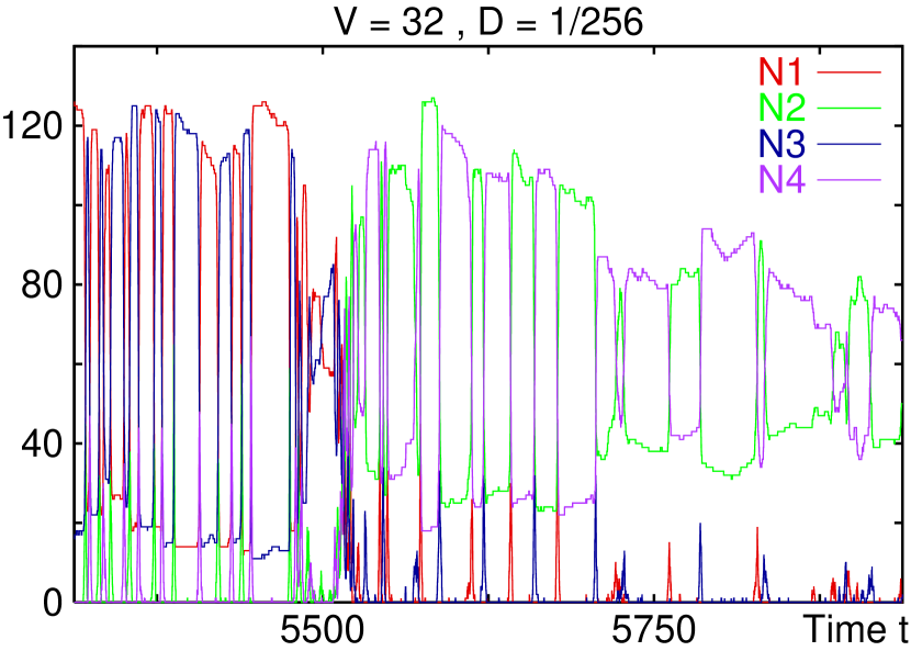
Figure 1: (color) Time series of the number of molecules $N_{i}(t)$, for $D=1/256,V=32$. Either 1-3 or 2-4 rich state is stabilized. Successive switches appear between $N_{1}>N_{3}$ and $N_{3}>N_{1}$ states with $N_{2},N_{4}\approx 0$. Here a switch from 1-3 rich to 2-4 rich state occurs around $t=5500$.

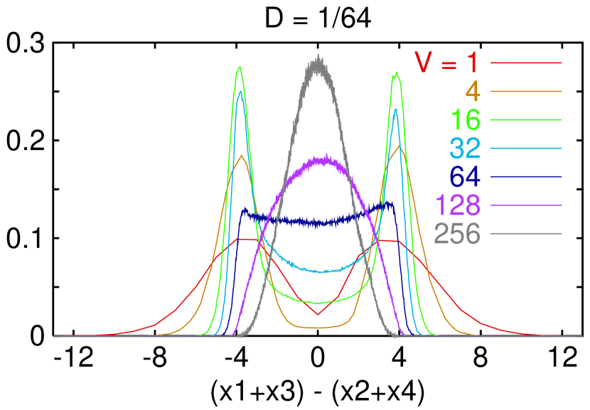
Figure 2: (color) The probability distribution of $z\equiv(x_{1}+x_{3})-(x_{2}+x_{4})$, sampled over $2.1$ – $5.2\times 10^{6}$ steps. $D=1/64$. For $V\geq 128$, $z$ has a distribution around 0, corresponding to the fixed point state $x_{i}=s(=1)$. For $V\leq 32$, the distribution has double peaks around $z\approx\pm 4$, corresponding to the state $N_{1},N_{3}\gg N_{2},N_{4}(\approx 0)$ or the other way round. The double-peak distribution is sharpest around $V=16$, and with the further decrease of $V$, the distribution is broader due to finite-size fluctuations.

The stability of this state is understood as follows. Consider the case with 1-3 rich and $N_{2}=N_{4}=0$. When one (or few) $X_{2}$ molecules flow in, $N_{2}$ increases, due to the autocatalytic reaction. Then $X_{3}$ is amplified, and since $N_{2}$ is not large, $N_{2}$ soon comes back to 0 again. In short, switch from $(N_{1},0,N_{3},0)$ to $(N_{1}-\Delta,0,N_{3}+\Delta+1,0)$ occurs with some $\Delta$, but the 1-3 rich state itself is maintained. In the same manner, this state is stable against the flow of $X_{4}$. The 1-3 rich state is maintained unless either $N_{1}$ or $N_{3}$ is close or equal to 0, and both $X_{2}$ and $X_{4}$ molecules flow in within the switch time. Hence the 1-3 rich state (as well as 2-4 rich state, of course) is stable as long as the flow rate is small enough.

Within a temporal domain of 1-3 rich state, switches occur to change from $(N_{1},N_{3})\rightarrow(N_{1}^{\prime},N_{3}^{\prime})$. In Fig. 3, we have plotted the probability density for the switch from $N_{1}\rightarrow N_{1}^{\prime}$ when a single $X_{2}$ molecule flows in, amplified, and $N_{2}$ comes back to 0, by fixing $N_{1}+N_{3}=N_{ini}$ at 256 initially. (We assume no more flow. Hence $N_{1}^{\prime}+N_{3}^{\prime}=N_{ini}+1$). The peak around $N_{1}^{\prime}\approx N_{1}+1$ means the reaction from $N_{2}$ to $N_{3}$ before the amplification, while another peak around $N_{1}^{\prime}\approx N_{3}=N_{ini}-N_{1}$ shows the conversion of the numbers through the amplification of $X_{2}$ molecules. Indeed, each temporal domain of the 1-3 rich state consists of successive switches of $(N_{1},N_{3})\rightarrow\approx(N_{3},N_{1})$, as shown in Fig. 1. Since molecules diffuse out or in randomly besides this switch, the difference between $N_{1}$ and $N_{3}$ is tended to decrease. On the other hand, each 1-3 rich state, when formed, has imbalance between $N_{1}$ and $N_{3}$, i.e., $N_{1}\gg N_{3}$ or $N_{1}\ll N_{3}$, since, as in Fig. 1, the state is attracted from alternate amplification of $X_{i}$, where only one type $i$ of molecules has $N_{i}\gg 1$ and 0 for others. However, the destruction of the 1-3 rich state is easier if $N_{1}\gg N_{3}$ or $N_{1}\ll N_{3}$, as mentioned. Roughly speaking, each 1-3 rich state starts with a large imbalance between $N_{1}$ and $N_{3}$, and continues over a long time span, if the switch and diffusion lead to $N_{1}\approx N_{3}$, and is destroyed when the large imbalance is restored. Indeed, we have plotted the distribution of $y\equiv x_{1}-x_{3}+x_{2}-x_{4}$, to see the imbalance for each 1-3 rich or 2-4 rich domain. This distribution shows double peaks clearly around $y\approx\pm 2.8,i.e.,(N_{1},N_{3})\approx(3.4V,0.6V),(0.6V,3.4V)$.

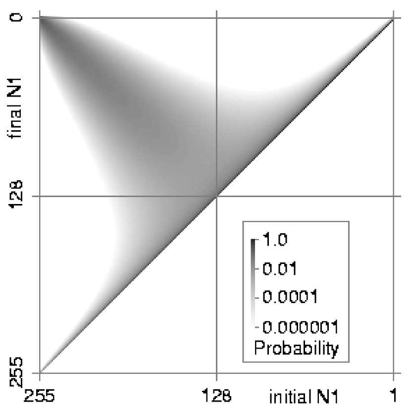
Figure 3: Probability density for the switch from $(N_{1},N_{3})$ to $(N_{1}^{\prime},N_{3}^{\prime})$ when a single $X_{2}$ molecule is injected into the system. $N_{1}+N_{3}=N_{ini}$ is fixed at 256 initially. There is no more flow and $N_{4}$ is always kept at 0, so that the switch is completed when $N_{2}$ comes back to 0, and $N_{1}^{\prime}+N_{3}^{\prime}=N_{ini}+1$. Probability to take $N_{1}^{\prime}$ is plotted against initial $N_{1}$.

Let us now discuss the condition to have the 1-3 or 2-4 rich state. First, the total number of molecules should be small enough so that the fluctuation from the state $N_{i}\approx N_{j}$ (for $\forall i,j$) may reach the state with $N_{i}\approx 0$. On the other hand, if the total number is too small, even $N_{1}$ or $N_{3}$ for the 1-3 rich state may approach 0 easily, and the state is easily destabilized. Hence the alternately rich state is stabilized only within some range of $V$.

Note also that our system has conserved quantities $\sum_{i}N_{i}$ (and $\sum_{i}logx_{i}$ in the continuum limit), if $D$ is set at $0$. Hence, as the diffusion rate gets smaller, some characteristics of the initial population are maintained over long time. Once the above 1-3 (or 2-4) rich state is formed, it is more difficult to be destabilized if $D$ is small. In Fig. 4, we have plotted the rate of the residence at 1-3 (or 2-4) rich state over the whole temporal domain, with the change of $V$. Roughly speaking, the state appears for $DV<1$ [18], while for too small $V$ (e.g., $V<4$), it is again destabilized by fluctuations. Although the range of the 1-3 rich state is larger for small $D$, the necessary time to approach it increases linearly with $V$. Hence it would be fair to state that properly small number of molecules is necessary to have the present state.

Figure 4: The rate of the residence at 1-3 (or 2-4) rich state over the whole temporal domain, plotted against $DV$ [18]. Here, the residence rate is computed as follows. As long as $N_{2}>0$ and $N_{4}>0$ are not satisfied simultaneously, over a given time interval (8.0; 2.5 times as long as the period of the oscillation around the fixed point at continuum limit), it is counted as the 1-3 rich state (2-4 rich state is defined in the same way) [23]. The residence rate is computed as the ratio of the fraction of the time intervals of 1-3 or 2-4 rich state to the whole interval. For small $D$, this switching state is observed even for a large number of molecules, say $N=4\times 10^{4}$, for $V=10^{4}$ at $D=10^{-6}$.

To sum up, we have discovered a novel state in reaction dynamics intrinsic to a small number of molecules. This state is characterized by alternately vanishing chemicals within an autocatalytic loop, and switches by a flow of single molecules [19]. Hence, this state generally appears for a system with an autocatalytic loop consisting of any even number of elements. With the increase of $k$, however, the globally alternating state all over the loop is more difficult to be reached. In this case, locally alternating states are often formed with the decrease of the system size (e.g., ‘2-4-6-8 rich’ and ‘11-13-15 rich’ states for $k=16$). This local order is more vulnerable to the flow of molecules than the global order for the $k=4$ loop.

On the other hand, for $k=3$, two of the chemical species start to vanish for small $V$, since any pair of different chemical species can react so that one chemical species is quickly absorbed into the other. This state of single chemical species, however, is not stable by a flow of a single molecule. Indeed, no clear ‘phase transition’ is observed with the decrease of $V$.

Although in the present Letter we have studied the case with $s_{i}=s$, we have also confirmed that the present state with alternately vanishing chemical species is generally stabilized for small $V$, even if $s_{i}$ or $r_{i}$ or $D_{i}$ are not identical.

Last, we make a remark about the signal transduction in a cell. In a cell, often the number of molecules is small, and the cellular states often switch by a stimulus of a single molecule [1]. Furthermore, signal transduction pathways generally include autocatalytic reactions. In this sense, the present stabilization of the alternately rich state as well as a single-molecule switch may be relevant to cellular dynamics. Of course, one may wonder that the present mechanism is too ‘stochastic’. Then, use of both the present mechanism and robustness by dynamical systems [20, 21] may be important. Indeed, we have made some preliminary simulations of complex reaction networks. Often, we have found the transition to a new state at a small number of molecules, when the network includes the autocatalytic loop of 4 chemicals as studied here [22]. Hence the state presented here is not restricted to this specific reaction network, but is observed in a class of autocatalytic reaction network. Furthermore switches between different dynamic states (limit cycles or chaos) are possible when the number of some molecules (that are not directly responsible to the switch) is large enough. The ‘switch of dynamical systems’ by the present few-number-molecule mechanism will be an important topic to be pursued in future.

We would like to thank C. Furusawa, T. Shibata and T. Yomo for stimulating discussions. This research was supported by Grants-in-Aid for Scientific Research from the Ministry of Education, Science, and Culture of Japan (Komaba Complex Systems Life Science Project).

References

- [1] B. Alberts, D. Bray, J. Lewis, M. Raff, K. Roberts and J. D. Watson, The Molecular Biology of the Cell (Garland, New York, 3rd ed., 1994).
- [2] H. H. McAdams and A. Arkin, Trends Genet. 15, 65 (1999).
- [3] F. Rieke and D. A. Baylor, Revs. Mod. Phys. 70, 1027 (1998).
- [4] N. G. van Kampen, Stochastic processes in physics and chemistry (North-Holland, rev. ed., 1992).
- [5] G. Nicolis and I. Prigogine, Self-Organization in Nonequilibrium Systems (John Wiley, 1977).
- [6] W. Horsthemke and R. Lefever, Noise-Induced Transitions, edited by H. Haken (Springer, 1984).
- [7] K. Matsumoto and I. Tsuda, J. Stat. Phys. 31, 87 (1983).
- [8] K. Wiesenfeld and F. Moss, Nature 373, 33 (1995).
- [9] B. Hess and A. S. Mikhailov, Science 264, 223 (1994); J. Theor. Biol. 176, 181 (1995).
- [10] P. Stange, A. S. Mikhailov and B. Hess, J. Phys. Chem. B 102, 6273 (1998); 103, 6111 (1999); 104, 1844 (2000).
- [11] D. A. Kessler and H. Levine, Nature 394, 556 (1998).
- [12] M. Eigen, P. Schuster, The Hypercycle (Springer, 1979).
- [13] M. Delbruck, J. Chem. Phys. 8, 120 (1940).
- [14] In a cell, reaction often takes place at a localized part of a cell. In this case, the volume in our model does not necessarily represent the whole cell volume, but the volume of such localized region.
- [15] One might assume the choice of the diffusion flow proportional to , considering the area of surface. Here we choose the flow proportional to , to have a well-defined continuum limit (eq.(1)) for . At any rate, by just re-scaling , the present model can be rewritten into the case with , for finite . Hence the result here is valid for the (and other) cases.
- [16] For small value, there appears deviation from this estimate. At any rate, the average number decreases monotonically with , and for , it goes to zero.
- [17] One may assume that a similar switch could exist in an equilibrium system due to a finite-size effect, e.g., in a small magnetic system with two ordered states of spins up and down. There, the two ordered states exist in the continuum (thermodynamic) limit. In contrast, the present ‘1-3 rich’ and ‘2-4 rich’ states to be switched do not exist in the continuum limit, but appear only through the discreteness of the number of molecules (and non-equilibrium dynamics allowing for oscillatory relaxation).
- [18] As shown in Fig. 4, there is a deviation from the scaling by . All the data are fit much better either by or by . At the moment we have no theory which form is justified.
- [19] The present transition does not require any details of a cell, but only chemical reactions within a small system surrounded by a permeable membrane. Hence, it can be experimentally verified by studying autocatalytic chemical reactions within a very small container, for example, within an artificially synthesized liposome.
- [20] K. Kaneko and T. Yomo, Bull. Math. Biol. 59, 139 (1997); J. Theor. Biol. 199, 243 (1999).
- [21] C. Furusawa and K. Kaneko, Bull. Math. Biol. 60, 659 (1998); Phys. Rev. Lett. 84, 6130 (2000).
- [22] Stability of the alternately rich state also depends on the network structure, i.e., arrows coming in and out from the autocatalytic loop of 4 chemicals.
- [23] This estimate includes the case in which only one species exists, and gives an overestimate for very small V.