HIGHER DIPOLE BANDS IN THE NLC ACCELERATING STRUCTURE

Abstract

We show that scattering matrix calculations for dipole modes between 23-43 GHz for the 206 cell detuned structure (DS) are consistent with finite element calculations and results of the uncoupled model. In particular, the rms sum wake for these bands is comparable to that of the first dipole band. We also show that for RDDS1 uncoupled wakefield calculations for higher bands are consistent with measurements. In particular, a clear 26 GHz signal in the short range wake is found in both results.

1 INTRODUCTION

In the Next Linear Collider (NLC)[1], long trains of intense bunches are accelerated through the linacs on their way to the collision point. One serious problem that needs to be addressed is multi–bunch, beam break–up (BBU) caused by wakefields in the linac accelerating structures. To counteract this instability the structures are designed so that the dipole modes are detuned and weakly damped. Most of the effort in reducing wakefields, however, has been focused on modes in the first dipole passband, which overwhelmingly dominate. However, with a required reduction of about two orders of magnitude, one wonders whether the higher band wakes are sufficiently small.

For multi-cell accelerating structures higher band dipole modes can be obtained by several different methods. These include the so-called “uncoupled” model, which does not accurately treat the cell-to-cell coupling of the modes[2], an open–mode, field expansion method[3], and a finite element method employing many parallel processors[4]. (Note that the circuit approaches[5][6] do not lend themselves well to the study of higher bands.) A scattering matrix (S-matrix) approach can naturally be applied to cavities composed of a series of waveguide sections[7], such as a detuned structure (DS), and such a method has been used before to obtain first band modes in detuned structures[8][9]. Such a method can also be applied to the study of higher band modes.

In this report we use an S-matrix computer program[10][11] to obtain modes of the 3rd to the 8th passbands—ranging from 23-43 GHz—of a full 206–cell NLC DS accelerating structure. We then compare our results with those of a finite element calculation and those of the uncoupled model. Next we repeat the uncoupled calculation for the latest version of the NLC structure, the rounded, detuned structure (RDDS1). Finally, we compare these results with those of the DS structure and with recent wakefield measurements performed at ASSET[12].

2 S-MATRIX WAKE CALCULATION

Let us consider an earlier version of the NLC accelerating structure, the DS structure. It is a cylindrically–symmetric, disk–loaded structure operating at X-band, at fundamental frequency $f_{0}=11.424$ GHz. The structure consists of 206 cells, with the frequencies in the first dipole passband detuned according to a Gaussian distribution. Dimensions of representative cells are given in Table 1, where $a$ is the iris radius, $b$ the cavity radius, and $g$ the cavity gap. Note that the structure operates at $2\pi/3$ phase advance, and the period $p=8.75$ mm.

Table 1: Cell dimensions in the DS structure.

cell#	a [cm]	b [cm]	g [cm]
1	.5900	1.1486	.749
51	.5214	1.1070	.709
103	.4924	1.0927	.689
154	.4660	1.0814	.670
206	.4139	1.0625	.629

For our S-matrix calculation we follow the approach of Ref. [11]: A structure with $M$ cells is modeled by a set of $2M$ joined waveguide sections of radii $a_{m}$ or $b_{m}$, each filled with a number of dipole TE and TM waveguide modes. First the S-matrix for the individual sections is obtained, and then, by cascading, the S-matrix for the composite structure is found. Using this matrix, the real part of the transverse impedance $R_{\perp}$ at discrete frequency points is obtained. We simulate a structure closed at both ends, and one with no wall losses. For such a structure $R_{\perp}$ consists of a series of infinitesimally narrow spikes. To facilitate calculation we artificially widen them by introducing a small imaginary frequency shift, one small compared to the minimum spacing of the modes. To facilitate comparison with the results of other calculation methods, we fit $R_{\perp}(\omega)$ to a sum of Lorentzian distributions, from which we extract the mode frequencies $f_{n}$ and kick factors $k_{n}$. Knowing these the wakefield is given by

$$W_{\perp}(s)=2\sum_{n}k_{n}\sin(2\pi f_{n}s/c)\,e^{-\pi f_{n}s/Q_{n}c}\quad,$$ (1)

with $s$ the distance between driving and test particles, $c$ the speed of light, and $Q_{n}$ the quality factor of mode $n$.

For our DS S-matrix calculation we approximate the rounded irises by squared ones. We use 15 TE and 15 TM waveguide modes for each structure cavity region, and 8 TE and 8 TM modes for each iris region. Our imaginary frequency shift is 1.5 MHz. Our resulting kick factors, for frequencies in the 3rd–8th passbands (23–43 GHz), are shown in Fig. 1. (Note that the effect of the 2nd band modes is small and can be neglected.) In Fig. 1 we show also, for comparison, the results of a finite element calculation of the entire DS structure[4], an earlier calculation that, however, does include the rounding of the irises.

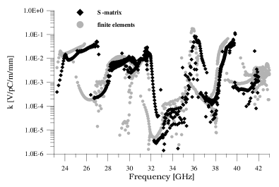
Figure 1: Results for the DS structure as obtained by the S-matrix and the finite element approaches. Note that the dimensions in the two cases differ slightly.

We note from Fig. 1 that the agreement in the results of the two methods is quite good, taking into account the difference in geometries. We see that the strongest modes are ones in the 3rd band (24-27 GHz), the 6th band (35-37 GHz), and the 7th band (38-40 GHz), with peak values of $k=.04$, .08, and .08 V/pC/mm/m, respectively (which should be compared to .4 V/pC/mm/m for 1st band modes). However, thanks to the variation in $a$ (for the 7th band) and $g$ (for the 3rd and 6th bands), these bands are seen to be significantly detuned, or spread in frequency. Another comparison is to take $2\sum k_{n}$ for the bands, a quantity that is related to the strength of the wakefield for $s\sim 0$, before coupling or detuning have any effect. For our S-matrix calculation for bands 3-8 this sum equals 19, for the finite element results 21 V/pC/mm/m (for the first two bands it is 74 V/pC/mm/m).

It is also necessary to know the mode $Q$’s to know the strength of the wakefield at bunch positions. A pessimistic estimate takes the natural $Q$’s due to Ohmic losses in the walls for the closed structure. Assuming copper walls these $Q$’s are very high for some of these higher band modes ($>10000$). In the real structure, however, the $Q$’s can be much less, depending on the coupling of the modes to the beam tubes and the fundamental mode couplers, effects that in principle can be included in the S-matrix calculation. In practice, however, these calculations are very difficult.

3 THE UNCOUPLED MODEL

The uncoupled model is a relatively simple way of estimating the impedance and the wake. It can be applied easily to higher band modes (unlike the circuit models) and to structures that are not composed of a series of waveguide sections (unlike the S-matrix approach). However, since it does not accurately treat the cell-to-cell coupling of the modes, it does not give the correct long time behavior of the wakefield.

The wakefield, according to the uncoupled model, is given by an equation like Eq. 1, except that the sum is over the number of cells $M$ times the number of bands $P$, and the mode frequencies and kick factors are replaced by ${\tilde{f}}_{pm}$ and ${\tilde{k}}_{pm}$, which represent the synchronous mode frequencies and kick factors, for band $p$, of the periodic structure with dimensions of cell $m$ of the real structure. For our uncoupled calculation we obtain the ${\tilde{f}}_{pm}$ and ${\tilde{k}}_{pm}$ for a few representative cells of the structure using an electromagnetic field solving program, such as MAFIA[13], and obtain them for the rest by interpolation.

In Fig. 2 we plot again the kick factors obtained by the S-matrix approach for the DS structure (rectangular irises), but now compared to the results of the uncoupled model applied to the same structure. The agreement is better than in Fig. 1. We expect the kick factors for the two methods to be somewhat different, due to the cell-to-cell coupling, but the running sum of kick factors, which is related to the short-time wake, should be nearly the same. The running sum, beginning at 20 GHz, of the two calculations is plotted in Fig. 3. We note that agreement, indeed, is very good.

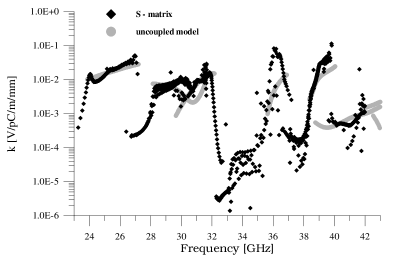
Figure 2: Kick factor comparison for the DS structure (square irises).

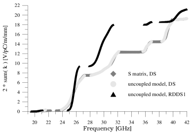
Figure 3: Running sum of kick factor comparison.

In Fig. 4 we plot the amplitude of the dipole wakes, for the frequency range 23-43 GHz only, of the DS structure (with squared irises), as obtained by the two approaches. (Here $Q$ has been set to 6500, appropriate for copper wall losses for the 15 GHz passband). Note that horizontal axis of the graph is $\sqrt{s}$ in order to emphasize the wake over the shorter distances. Far right in the plot is equivalent to $s=80$ m, the NLC bunch train length. We note that the initial drop-off and the long-range wake are very similar, though there is some difference in the region of 1-10 m. The amplitude at the origin, 20 V/pC/mm/m, is small compared to 78 V/pC/mm/m for the first dipole band, but the longer time typical amplitude of $\sim 1$ V/pC/mm/m is comparable to that of the first band. The rms of the sum wake, $S_{rms}$, an indicator of the strength of the wake force at the bunch positions, for the higher bands is .5 V/pC/mm/m, which is comparable to that of the first dipole band. Depending on the external $Q$ for the structure, however, $S_{rms}$ for the higher bands may in reality be much smaller.

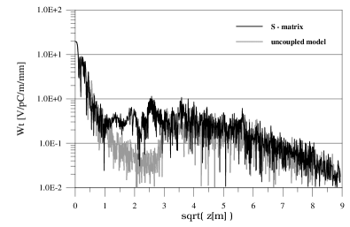
Figure 4: Comparison of wakefields (23-43 GHz frequency range only) for the DS structure (square irises).

The latest version of the NLC structure is RDDS1 which has rounded irises as well as rounded cavities. As such it is difficult to calculate using the S-matrix approach. We have not yet done a parallel processor, finite element calculation, but we have done an uncoupled one. The sum of the kick factors of the result is given also in Fig. 3 above. Although the running sums at 42 GHz for DS and RDDS1 are very similar, at lower frequencies the curves are quite different. In particular, the 3rd band modes ($\sim 26$ GHz) appear to be less detuned for RDDS1, the 4th and 5th band modes (27-31 GHz) are stronger, though still detuned, and between 32-40 GHz there is very little impedance.

4 ASSET MEASUREMENTS

Measurements of the wakefields in RDDS1 were performed at ASSET[12]. In Figs. 5,6 we present results for the vicinity of .7 and 1.4 nsec behind the driving bunch. To study the higher band wakes we have removed the 15 GHz component from the data in the plots. The remaining wake was fit to the function $A\sin(2\pi F+\Phi)$ with $A$, $F$, and $\Phi$ fitting parameters. This fit, along with the 3rd band component of the uncoupled model results ($\sim 26$ GHz), are also given in the figures. At .7 nsec this component is clearly seen in the data, and the amplitude and phase are in reasonable agreement with the calculation. At 1.4 ns there is more noise, though the 26 GHz component can still be seen.

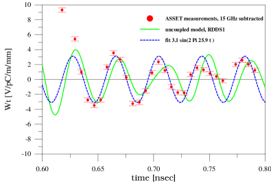
Figure 5: The measured wake function for RDDS1, with the 15 GHz component removed.

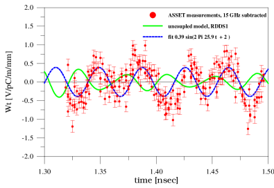
Figure 6: The measured wake function for RDDS1, with the 15 GHz component removed.

References

- [1] NLC ZDR Design Report, SLAC Report 474, 589 (1996).
- [2] K. Bane, et al, EPAC94, London, 1994, p. 1114.
- [3] M. Yamamoto, et al, LINAC94, Tsukuba, Japan, 1994, p. 299.
- [4] X. Zhan, K. Ko, CAP96, Williamsburg, VA, 1996, p. 389.
- [5] K. Bane and R. Gluckstern, Part. Accel., 42, 123 (1994).
- [6] R. M. Jones, et al, Proc. of EPAC96, Sitges, Spain, 1996, p. 1292.
- [7] J.N. Nelson, et al, IEEE Trans. Microwave Theor. Tech., 37, No.8, 1165 (1989).
- [8] U. van Rienen, Part. Accel., 41, 173 (1993).
- [9] S. Heifets and S. Kheifets, IEEE Trans. Microwave Theor. Tech., 42, 108 (1994).
- [10] V.A. Dolgashev, “Calculation of Impedance for Multiple Waveguide Junction,” presented at ICAP’98, Monterey, CA, 1998.
- [11] V. Dolgashev et al, PAC99, New York, NY, 1999, p. 2822.
- [12] C. Adolphsen et al., PAC99, New York, NY, 1999, p. 3477.
- [13] The CST/MAFIA Users Manual.