Some possibilities for laboratory searches for variations of fundamental constants

Abstract

We consider different options for the search for possible variations of the fundamental constants. We give a brief overview of the results obtained with several methods. We discuss their advantages and disadvantages with respect to simultaneous variations of all constants in both time and space in the range $10^{8}-10^{10}$ yr. We also suggest a few possibilities for the laboratory search. Particularly, we propose some experiments with the hyperfine structure of hydrogen, deuterium and ytterbium–171 and of some atoms with a small magnetic moment. Other suggestions are for some measurements of the fine structure associated with the ground state. Special attention is paid to the interpretation of the hfs measurements in terms of variations of the fundamental constants.

1 Introduction

There is no physical reason to expect that the “fundamental constants” are really constant quantities. Indeed, their variations have to have a cosmological scale. Since the publishing of a famous Dirac paper [2] a number of different hypotheses on their possible variations have been suggested as well as a number of trial to search for these. A review of old models and searches could be found e. g. in Ref. [3]. We live in an expanding universe and an accepted contemporary picture of the history of our universe assumes that there were a few phase transitions with spontaneous breaking of some symmetries during the early stages of evolution (inflation model) [4].

We consider here only atomic and nuclear properties and the variations of the fundamental constants that can be determined from changes in such properties. We do not discuss variation of the gravitational constant (a review on that can be found in Refs. [3, 5]). There are two reasons for that. First of all, in looking for variations of nuclear and atomic properties (magnetic moments, masses, decay rates) it is not possible to consider strong, weak and electromagnetic effects independently. Next, from a theoretical point of view, we have to expect that the variations of strong, weak and electromagnetic coupling constants are strongly correlated. In contrast to that, any investigation for possible variations of the gravitational interaction can be done separately.

1.1 Variation of the constants and atomic spectroscopy

Any search for a possible variation of the fundamental constants can be actually performed measuring some atomic, molecular and nuclear properties and it is necessary to discuss relations between them. There are three very different kinds of atomic and molecular transitions, available for precision spectroscopy:

• Gross structure is associated with transitions between levels with different values of the principal number $n$. They have a scaling behaviour as $\alpha^{2}\,m_{e}\,c^{2}/h$ or $Ry$. It has to be remembered that for any atom with two or more electrons, one has to introduce an effective quantum number $n^{*}$, which is a function of the orbital momentum ($l$). The nonrelativistic behaviour $\alpha^{2}\,m_{e}\,c^{2}/h$ is actually associated with $n^{*}(l)$ and, hence, in non-hydrogen-like atoms, transitions between levels with different value of $l$ are also a part of the gross structure.

• Atomic fine structure, or separations of levels with the same $n^{*}(l)$ and different spin-orbit coupling (e. g. different $j$ or different sum of spin of valence electrons), has a scaling behaviour $\alpha^{4}\,m\,c^{2}/h$ or $\alpha^{2}\,Ry$. That is part of relativistic corrections, which have the same order of magnitude.

• Atomic hyperfine structure is a splitting due to a magnetic moment of the nucleus ($\mu$) and it is proportional to $\alpha^{4}\,m\,c^{2}/h\,(\mu/\mu_{\sc b})$ or $\alpha^{2}\,(\mu/\mu_{\sc b})\,Ry$.

Comparing frequencies with different scaling behaviour, one can look for variations of the fundamental constants and nuclear magnetic moments. An important part of those comparisons is the so-called absolute frequency measurements. An absolute measurement of a frequency is actually its comparison to the hfs of Cs, because of the definition of second via the Cs hfs interval

$$\nu_{\rm hfs}(^{133}{\rm Cs})=9\,9192\,631.770~{}{\rm kHz}\quad{\rm(exactly)}\,.$$ (1)

Another possibility is to study some corrections. E. g. the study of relativistic corrections to the atomic gross structure or hfs can yield to detection of possible variations of the fine structure constants, while investigations of the electronic-vibrational-rotational lines can give limitations for the variation of the proton-to-nuclear mass ratio. Due to the importance of the value in Eq.(1) let us to discuss corrections to the hfs in some detail. The value of the hyperfine splitting in an atomic state can be presented in the form

$$\nu_{\rm hfs}=c_{0}\,\alpha^{2}\,\frac{\mu}{\mu_{\sc b}}\,{\rm Ry}\,F_{\rm rel}(\alpha)\,,$$ (2)

where $\mu$ stands for the nuclear magnetic moment, $c_{0}$ is a constant specific for the atomic state and all dependence on $\alpha$ is contained in a function $F_{\rm rel}(\alpha)$, which is also specific for the state. The function is associated with the relativistic corrections and $F_{\rm rel}(0)=1$. The corrections are more important for high $Z$ and in the case of low $Z$ (e. g. for the hydrogen hfs) they are negligible.

1.2 Variable particle, atomic and nuclear properties

There are three possibilities for the variation of fundamental properties, which can be studied within spectroscopic methods:

• effects due to electromagnetic interactions and value of electromagnetic coupling constant $\alpha$ (study of $1s-2s$, comparison of the gross and fine structure, study of relativistic corrections);

• effects of quark-quark and quark-gluon strong interactions and nucleon properties like $\mu_{p}$, $\mu_{n}$, $m_{p}$ etc (study of the hfs of hydrogen and light nuclei, or molecular electronic-vibrational-rotational lines);

• nuclear properties (moments and masses) due to the structure of heavy nuclei. Some of those properties (like magnetic dipole and electric quadrupole moments) can be studied by means of atomic and molecular spectroscopy. Nuclear decay rates and scattering cross sections of nuclear collisions can be investigated by other methods.

We mainly consider here applications of the precision spectroscopy. Experiments with the hfs of heavy atoms (e. g. Cs, Rb, Yb⁺ or Hg⁺) cannot have any clear interpretation: any of the values are proportional to a non-relativistic matrix element, but with significant relativistic corrections (see Eq.(2)). The non-relativistic value is proportional to a magnetic moment of the nucleus, which includes the moments of one or two valence protons and neutrons and some contribution of an internal nuclear motion. The last is not a pure effect of the strong interactions and an influence of electromagnetic interactions can be estimated from the proton-neutron asymmetry.

If we keep in mind a general picture, we have to expect a kind of “grand unification” theory and there has to be some direct relations between coupling constants for weak, electromagnetic and strong interactions (see e. g. [6, 4]). Hence, all fundamental constants (i. e. $\alpha$, $\alpha_{\sc s}$ and $\alpha_{\sc w}$) are expected to vary within about the same rate. Indeed, different atomic, molecular or nuclear properties can have quite different sensitivities to variations of the coupling constants.

It is necessary to emphasise that it is incorrect to think that some values like proton-electron mass ratio or nuclear $g$-factor are expected to be relatively constant, while the electromagnetic coupling constant $\alpha$ varies, as is expected in the interpretation of some papers. The bare electron mass is a result of the interaction with the Higgs field [7] and it has significant quantum electrodynamical corrections due to the renormalization. The bare $u$- and $d$-quark masses also appear from the Standard model as a result of interaction with the Higgs sector and are a few Mev. However, the actual masses of the proton and neutron are determined by the masses of the constituent quarks, which are about 300 Mev and those values are completely a result of the dynamic effects of the QCD in a strong coupling range. The same is true with the proton and neutron magnetic moments. Such a value, appearing as a result of the strong interactions, is definitely a function of the strong coupling constant, which is expected to vary together with the electromagnetic and weak coupling constants.

Let us consider the electron mass in more detail. A standard interpretation of quantum electrodynamics (QED) is that it has to be possible to explain all low-energy (with respect to the Planck mass $M_{\sc p}$) physical phenomena, using only few effective low-energy parameters (like renormalized electron mass and charge etc). The origin of those values is not important. However, in the case of the search for variations of the constants it is necessary to study the origin of the low-energy parameters, like the electron mass. The bare electron mass $m_{0}$ is to be renormalized due to the QED effects. In the one-loop approximation on can find

$$m_{e}=m_{0}\left[1+\frac{3}{4}\,\frac{\alpha}{\pi}\,\ln\left(\frac{\Lambda}{m_{0}}\right)^{2}\right]\,,$$ (3)

where the $\Lambda$ is an effective cut-off of the ultraviolet divergence. If the cut-off is associated with the Planck scale $\Lambda=M_{\sc p}\sim 1.2\cdot 10^{19}~{}{\rm Gev}\sim 2.4\cdot 10^{21}~{}m_{e}$, the logarithmic correction is about 20% of the leading term. One can see that, even in the case of a constant value of $m_{0}$, the actual electron mass $m_{e}$ has to vary with $\alpha$.

From a theoretical point of view we can rather expect a primary variation of some parameters which are not visible directly in our low-energy world and this forces some secondary variations of the coupling constants. E. g. in the inflatory universe (see Ref. [4] for detail), some effective Higgs potentials depend on the average temperature, which is a function of the time. That have led to some phase transition in the past, when the hot universe was cooling. We think that even in our “cool” universe we can expect some slow time variation of those Higgs potentials and perhaps their long-scale space variation. The variations of the constants is to be a direct consequence of that.

Another and more sophisticated idea [8] was proposed due to the so-called Kaluza-Klein theories, which are associated with a world of $4+N$ dimensions. In contrast to “our” 4 dimensions, the extra spatial $N$ dimensions form a compact manifold with a radius $R_{\sc kk}$ about Planck length ($\sim 10^{-33}$ cm). While our four dimensional universe is expanding, Marciano suggested that value of $R_{\sc kk}$ is also not constant. However, in the Kaluza-Klein theory this value is associated with the coupling constants of our world.

So, we expect that the variation of different coupling constants has to have the same scale. However, it is necessary to remember that due to the strong coupling any effective parameters coming from the strong interactions, can have a kind of random variation. We cannot often know which quantity is varied more (or less) rapidly than the fundamental constants. That is why we have to try with several ways as different as possible.

No model on a possible dependence of the values of the fundamental constants has not been assumed in our paper. However, we must underline, that we consider a picture of simultaneous variations of all coupling constants, which particularly determine all property of particles, nuclei, atoms and molecules.

We have not yet specified a term “variations”. To our mind there are actually two possibilities for those:

• A time and/or space variation over all the universe with a cosmological scale ($T\sim 10^{10}$ yr and $L\sim c\cdot 10^{10}$ yr).

• Time and/or space fluctuations over some less, but significantly cosmological, scale ($T\sim 10^{8}-10^{9}$ yr and $L\sim c\cdot(10^{8}-10^{9})$ yr).

Such a fluctuation of the gravitation interaction was considered [9, 10, 11, 12, 13, 14] due to a periodicity in the galaxies distributions in the direction of the Galactic north and south poles [15]. The fluctuations of gravitation is also one of the explanations of possible variations to the solar year [13].

The variation can be induced e. g. by cooling of the universe and a variation of some effective Higgs potentials. We have no a priori estimation for the speed of the variations. We expect the cosmological time and space scale ($T$ and $L$), but we have no idea on the amplitude of the possible variations. The expected amplitude particularly depends on our assumption if we expect some kind of a primary direct variation of the constants, or their variations are a consequence of variations of some other parameters. E. g. let us pretend that the primary variation is due to the compactification radius $R_{\sc kk}$ and there is no variation of the coupling constants on the unperturbed level. Nevertheless, the variations have to appear due to the renormalization and the time-dependence is to be of the relative order $\alpha\ln{R_{\sc kk}(t)}$. Particularly, following QED one can find in the one-loop approximation an expression for the fine structure constant

$$\alpha=\frac{\alpha_{0}}{1-\frac{1}{3}\,\frac{\alpha_{0}}{\pi}\,\sum_{j}{c_{j}}\,q_{j}^{2}\,\ln\bigl{(}\Lambda/m_{j}\bigr{)}^{2}}~{},$$ (4)

where $\Lambda\simeq\hbar/cR_{\sc kk}$, the sum is over all fundamental charged particles (leptons, quarks, $W$-bosons, Higgs particles etc), $m_{j}$ stands for their masses, $q_{j}$ is for their charges. The coefficient $c_{j}$ is dependent on their spin and particularly for 1/2 it is equal to one. A significant variation of $R_{\sc kk}$ (e. g. 1%) can induce a variation of $\alpha$ only on a level between $10^{-4}-10^{-5}$. The extra $\alpha$ and the logarithm reduce the amplitude of the variation dramatically. However, it is important to note, that the variation of the mass in Eq.(3) with $\Lambda=R_{\sc kk}(t)$ and of the charge in Eq.(4) are to be of the same origin and of about the same order. That example shows that the variation $\Delta\alpha/\alpha$ can be small and that the mass variation $\Delta m/m$ and the coupling constant variation can be of the same order and vary simultaneously. Actually comparing Eqs.(3) and (4) one can note that the variation of the mass can be larger, smaller or of the same order of magnitude as the variation of the coupling constant. Mass variations smaller or of the same order as the coupling constant have been discussed above. The larger mass variation can appear if we suggest that there is no direct variation of the coupling constants, but the masses vary e. g. due to some variation of the effective Higgs potential of the Standard Model. The $\alpha$-variation has to appear from Eq.(4) because of the $m$-variation in the logarithm. We conclude that a priori it is not feasible to dismiss the mass variation and to consider only varying coupling constants.

2 Non-laboratory search for variations of the fundamental constants

2.1 Geochemical data and nuclear properties

Nuclear reactions (collisions, decay etc) often involve some relatively small differences of large contributions. E. g. to understand if any isotope is stable for a particular channel of decay, one has to compare the initial and final binding energy. A problem of the stability is a problem of this difference, which is sometimes quite small. Relatively small shifts in particle masses or coupling constants can make the decay of a stable isotope possible, or disturb an allowed decay. The variation of the coupling constant of strong, electromagnetic or weak interactions can be weakly limited, but the geochemical estimations take advantage of long term comparisons. The study of the abundance of some isotopes allows one to make a comparisons over a geophysical scale of $10^{9}$ yr.

2.1.1 Geochemical data

Some estimations of possible variations of the coupling constants of strong, weak and electromagnetic interactions from geophysical, or rather, geochemical data were performed in Refs. [16, 17, 19, 18, 20, 3, 22, 23, 24] (see review in Refs. [3, 5] for more references). Some examinations also include data on the abundance of some isotopes in the meteorites, and so the results are, in part, astrochemical ones.

The typical limits are

$$\frac{1}{\alpha}\,\frac{\partial\alpha}{\partial t}<5\cdot 10^{-13}-3\cdot 10^{-15}~{}{\rm yr}^{-1}\,,$$

$$\frac{1}{\alpha_{\sc s}}\,\frac{\partial\alpha_{\sc s}}{\partial t}<5\cdot 10^{-11}-2\cdot 10^{-11}~{}{\rm yr}^{-1}$$

and

$$\frac{1}{\alpha_{\sc w}}\,\frac{\partial\alpha_{\sc w}}{\partial t}<10^{-10}~{}{\rm yr}^{-1}\,.$$ (5)

One problem with the interpretation of those data is the authors assumed of Refs. [3, 19, 21, 22, 23] that only coupling constants vary, while the masses of the proton, the neutron and the electron are constant. Conversely, we expect those to vary as well, and some nuclear effects are sensitive to that variation. Particularly, the $\beta$-decay must be very sensitive to their difference

$$m_{n}-m_{p}-m_{e}\,.$$

We should remember that often the violation of the isotopic invariance and particularly the small difference of the proton and neutron masses

$$\frac{m_{n}-m_{p}}{m_{p}}\sim 0.14\%$$ (6)

is associated with electromagnetic effects.

Next, it was assumed that it is possible to look for a variation of some particular constant (e. g. $\alpha$) while others are really constant. We cannot accept such an evaluation, but nevertheless we would like to underline, that the nuclear property can be very sensitive to a variation of the constants, because the decay rates are strongly dependent on the transition energy, which is actually a small difference of two larger energies of initial and final states. Both include contributions of the electromagnetic interactions and the difference can be quite sensitive to these.

Another important problem is timing. Geochemical clocks are based on the study of the abundance of some long-living isotopes and others associated with them. A long lifetime is a result of a small value of the transition either matrix element or energy. Both, being small, are sensitive to the same variation of the constants. To the best of our knowledge there have been no discussions on a correlation between the clock and the variation.

2.1.2 Geochemical data from Oklo reactor

Shlyakhter [25] introduced two important elements in the study of nuclear reactions. First, he pointed out that laboratory investigations of nuclear property can also give reasonable limitations (see section 3.1). His other idea was due to the recently discovered Oklo Fossil reactor in Gabon (West Africa). That is a natural fission reactor (see review in Refs. [26, 27]), and conditions for its existence are very narrow. Investigating those conditions and the local abundance of different isotopes (particularly Sm) it is possible to derive some limitations such that it had operated 1.7 billions years ago for a period from 0.6 to 1.5 millions years. The limits from Ref. [25] are

$$\frac{1}{\alpha}\,\frac{\partial\alpha}{\partial t}<1\cdot 10^{-17}~{}{\rm yr}^{-1}\,,$$

$$\frac{1}{\alpha_{\sc s}}\,\frac{\partial\alpha_{\sc s}}{\partial t}<1\cdot 10^{-18}~{}{\rm yr}^{-1}$$

and

$$\frac{1}{\alpha_{\sc w}}\,\frac{\partial\alpha_{\sc w}}{\partial t}<4\cdot 10^{-12}~{}{\rm yr}^{-1}\,.$$ (7)

One evidence of the operation of the nuclear reactor in the past was isotope compositions of some elements like samarium, europium and gadolinium. Some of their isotopes (¹⁴⁹Sm, ¹⁵¹Eu, ¹⁵⁵Gd and ¹⁵⁷Gd) are strong neutron absorbers and they have been found in very small quantities with respect to the natural abundance. They have simply been burned by the flux of thermal neutrons. A study of such isotopes can give information on the fundamental constants at a time when the fossil reactor was operating. Particularly, the limitations in Eqs.(2.1.2) have appeared because of the resonance

$${}^{149}{\rm Sm}+n\to{}^{150}{\rm Sm}+\gamma\,,$$ (8)

which has an energy of only 97.3 meV. Two isotopes of samarium (147 and 149) have been studied. The halftime of the isotopes is presented in Table 1. The cross sections of reaction in Eq.(8) and a similar one for

$${}^{147}{\rm Sm}+n\to{}^{148}{\rm Sm}+\gamma\,,$$ (9)

differ by about two orders of magnitude because of the resonance. Studying the ${}^{147}{\rm Sm}/{}^{149}{\rm Sm}$ ratio one can deduce a possible variation of the position of the resonance from when the reactor was operating to the present day. The strength of the limitations in Eqs.(2.1.2) has three reasons:

• the sensitivity of the abundance of samarium isotopes to the position of the resonance;

• the fact that the resonance energy ($\sim 100$ meV) has to be compared with a well of the nuclear potential ($\sim 50$ Mev) i. e. it is $5\cdot 10^{8}$ times larger then the energy;

• large time separation ($\sim 2\cdot 10^{9}$ yr).

Isotopes	Halftime	Natural	Neutron separation
		abundance	energy $S_{n}$ [keV]
147	$1.06\cdot 10^{11}$ yr	15.0%	6342(3)
148	$7\cdot 10^{13}$ yr	11.3%	8141.5(6)
149	$>2\cdot 10^{15}$ yr	13.8%	5871.6(9)
150	stable	7.4%	7985.7(7)

Table 1: Properties of some samarium isotopes.

After publication of Ref. [25] the Oklo data have been re-evaluated by a number of authors [27, 29, 5, 30, 31]. The evaluations were concentrated on the samarium abundance. Particularly, it was pointed out in Ref. [31] that for the limitations for the strong coupling constant it is unlikely to be appropriate to compare the position of the resonance to the well of the nucleon-nucleon potential, which is essentially of use only in the few-body problem. In the case of many-body effect (like the resonance) it was suggested to consider a neutron separation energy $S_{n}$ (see Table 1) as a characteristic reference value. The latter is 6–8 Mev and significantly smaller than the well ($\sim 50$ Mev).

Investigations of other isotopes were not as effective in setting limits. Some estimations due to europium were presented by Shlyakhter, while gadolinium was studied in Ref. [31]. But the studies did not yield such strong limitations as the investigations of the samarium isotopes.

Results for the variation of the fine structure constant from the Oklo reactor study are collected in Table 2. The most recent estimates are [30]

$$\frac{1}{\alpha}\,\frac{\partial\alpha}{\partial t}=-1.4(54)\cdot 10^{-17}~{}{\rm yr}^{-1}\,,$$

$$\frac{1}{\alpha_{\sc w}}\,\frac{\partial\alpha_{\sc w}}{\partial t}<1\cdot 10^{-11}~{}{\rm yr}^{-1}\,,$$ (10)

and [31]

$$\frac{1}{\alpha}\,\frac{\partial\alpha}{\partial t}<1.0\cdot 10^{-17}~{}{\rm yr}^{-1}\,,$$

$$\frac{1}{\alpha_{\sc s}}\,\frac{\partial\alpha_{\sc s}}{\partial t}<1.3\cdot 10^{-18}~{}{\rm yr}^{-1}\,.$$ (11)

Those results cannot be used directly, because of the same reasons as those for other geochemical data. Particularly, the timing was based on the abundance of strong absorbers of thermal neutrons and any influence of the variation of the constants on utilized cross sections was not investigated. Variation of the fine structure constant was analyzed only with respect to the static Coulomb interaction energy of the proton in the nucleus. However, we have to expect that a small part of the proton and neutron masses is a result of electromagnetic interactions and hence any variations of $\alpha$ lead to a shift in these masses and of the kinetic energy. Indeed only a small part of the kinetic energy is of this electromagnetic origin. However the entire kinetic energy is much larger than the static Coulomb interaction and eventually both electromagnetic contributions can be compatible.

Concerning two different recent results on the fine structure constant we note that in Ref. [31] more recent and accurate data on the samarium isotopic composition were used, while in Ref. [30] the estimation of the temperature was more secure. We also have to point out that it is unclear how much the neutron flux during the operation time of the reactor used in Refs. [30, 31] is sensitive to the possible variation of the constants. We think a proper way is to determine the flux and a possible variation simultaneously.

$\partial ln{\alpha}/\partial t$	Ref.
$<1\cdot 10^{-17}~{}{\rm yr}^{-1}$	[25]
$<2\cdot 10^{-18}~{}{\rm yr}^{-1}$	[29]
$-1.4(54)\cdot 10^{-17}~{}{\rm yr}^{-1}$	[30]
$<1.0\cdot 10^{-17}~{}{\rm yr}^{-1}$	[31]

Table 2: Limits for the $\alpha$ variation from Oklo.

2.1.3 Nucleosynthesis

Some estimations due to Big Bang nucleosynthesis have also been performed [32, 33] in a similar way to the geochemical study. A possible variation of the fine structure constant is not larger than $(1-2)\cdot 10^{-12}$ yr^-1. This cosmological estimate takes an advantage of a large time separation between the epoch of nucleosynthesis and the present day which is about the lifetime of the universe, i. e. about $10^{10}$ yr.

2.2 Astrophysical data

2.2.1 Absorption lines in quasar spectra

An advantage of astrophysical studies is a possibility of a long term comparison. A typical astrophysical time associated with extragalactic sources (quasars) is up to $10^{10}$ yr. Due to the long reference time the accuracy of spectroscopic measurements need not be high. It is also possible to look for corrections (like $m_{e}/m_{p}$ terms in H₂ spectrum). A key point of any astrophysical study is a comparison of observed lines with a data base of lines collected under laboratory conditions in order to determine a value of the redshift

$$\lambda_{\rm obs}=\lambda_{0}\big{(}1+z\big{)}$$ (12)

and, hence, a time separation between the epoch of the absorption and the epoch of the observation $t(z)$. This depends on the choice of evolution parameters of the universe and can vary by a factor two for the same $z$. When the lines are identified, one can try to interpret spectroscopic data in terms of variations of transition frequencies. It is quite important to determine the redshift and look for the variation simultaneously. When one does this separately it is equivalent to an assumption on the stability of particular transitions. E. g. in Ref. [34], the authors used the redshift from the observation of some astrophysical data on the hydrogen hfs line, and so they actually assumed within the evaluation that the $\alpha^{2}\mu_{p}/\mu_{\sc b}Ry$ is a stable value and this led to some misinterpretation.

A comparison of frequencies with different scaling behaviours is described in Sect. 1.2. Particularly, Savedoff [36] pointed out this application for the comparison of atomic lines. Thompson first noted that molecular spectra could be used to examine the variation of the nuclear masses [37]. An analysis of absorption lines of molecular hydrogen in a quasar spectrum can possibly provide a limit for the variation of the proton-to-electron mass ratio. Such an evaluation is based on the Born-Oppenheimer approximation of the molecular spectrum

$$\nu_{\rm mol}={\rm Ry}\left[c_{e}+c_{v}\left(\frac{m_{e}}{M}\right)^{1/2}+c_{r}\left(\frac{m_{e}}{M}\right)+\dots\right]\,,$$ (13)

where $c_{i}$ are dimensionless parameters of order ${\cal O}(1)$. The dominate term $c_{e}$ is determined by the electronic structure, the second is due to the vibrational excitations, while the third one is associated with the rotational levels. Comparing levels with the same electronic structure (the same $a$), it is possible to study two other terms and to limit the variation of the electron-to-proton mass ratio from the H₂ spectrum. Value $M$ is associated with some nuclear mass, particularly in the case of diatomic molecules it is the reduced mass of two nuclei. It is important for applications that the coefficients $c_{i}$ can be found both theoretically and experimentally. The latter is possible by studying different isotopes, particularly the reduced mass $M$ for H₂, HD, D₂ etc varies enough to allow this (see e. g. Ref. [34]).

An examination of the molecular lines, or a comparison of the rotational and vibrational transitions with the gross structure yields a variation of $m_{e}/m_{p}$. In contrast to this a comparison of the rotational terms to the hfs in the hydrogen atom yields a limit for the $\alpha^{2}\,g_{p}$ variation. Analysis of the molecular lines was performed in Ref. [38, 39], while in Refs. [40, 41, 34, 42, 35] the authors preferred to compare the rotational and vibrational transitions with the hfs of the hydrogen atom. The most accurate results are collected in Table 3.

A comparison of the gross structure to the fine structure of some ions presented in Refs. [43, 44, 45, 46, 47, 41, 34, 48, 39, 49, 50] gave limitations on the variations of $\alpha^{2}$. Variations of the same value can be found after studying the relativistic corrections. The most recent results were obtained in [51], where an evaluation of data for some of Fe⁺ and Mg⁺ lines was performed. The variation of the fine structure constant was obtained from a study of relativistic corrections, calculations for which were presented separately in Ref. [52, 53].

The hfs of atomic hydrogen was examined with respect to the gross structure in Refs. [44, 41] and with respect to the fine structure in Refs. [44, 34]. The former of those examinations is for possible variations of $\alpha^{2}\,(\mu_{p}/\mu_{\sc b})$, while the latter is for $\mu_{p}/\mu_{\sc b}$. The strongest astrophysical limitations are summarized in Table 3, where we give variations for actually measured values. References to previous, less precise results can be found in quoted articles and in Ref. [45].

Value	Ref.	$\partial\ln(<{\rm value}>)/\partial t$
		[yr-1]
$m_{e}/m_{p}$	[38]	$<3\cdot 10^{-13}$
$m_{e}/m_{p}$	[41]	$-0.8(35)\cdot 10^{-14}$
$m_{e}/m_{p}$	[48]	$<2\cdot 10^{-14}$
$m_{e}/m_{p}$	[39]	$9(6)\cdot 10^{-15}$
$\alpha^{2}$	[47]	$<6\cdot 10^{-14}$
$\alpha^{2}$	[46]	$<4\cdot 10^{-14}$
$\alpha^{2}$	[41]	$1.0(35)\cdot 10^{-14}$
$\alpha^{2}$	[34]	$<3\cdot 10^{-14}$
$\alpha^{2}$	[39]	$<5\cdot 10^{-15}$
$\alpha^{2}$	[51, 52]	$0.4(51)\cdot 10^{-15}$
$\alpha^{2}$	[49]	$<5\cdot 10^{-15}$
$\alpha^{2}\,g_{p}$	[34]	$<2\cdot 10^{-14}$
$\alpha^{2}\,g_{p}$	[35, 42]	$<2\cdot 10^{-15}$
$\alpha^{2}\mu_{p}/\mu_{\sc b}$	[44]	$<2\cdot 10^{-14}$
$\alpha^{2}\mu_{p}/\mu_{\sc b}$	[41]	$-1.0(13)\cdot 10^{-15}$

Table 3: Possible variations of the constants from astrophysics.

2.2.2 Background radiation

An analysis of microwave background radiation data to be obtained in the near future is expected to give a limitation for a variation of the fine structure constant of $10^{-12}-10^{-13}$ yr ^-1 [54, 55].

3 Laboratory search

The limitations from Eq.(2.1.2) and Table 3 are stronger than possible in any laboratory experiments. However, to our mind, the most reliable limitations can be achieved only under laboratory conditions and there are a few very different ways to determine limits for possible variations of the fundamental constants.

3.1 Laboratory nuclear data

As has been mentioned, Shlyakhter noted that the laboratory study of some nuclear properties can give reasonable limitations for variations of the constants [25]. He considered some very low-lying resonances, the energies of which are extremely small differences of large quantities and those must be sensitive to small variations of parameters. The positions of some of these resonances had been known with enough accuracy for about 10 years and an estimate

$$\frac{1}{\alpha_{\sc s}}\,\frac{\partial\alpha_{\sc s}}{\partial t}<4\cdot 10^{-12}~{}{\rm yr}^{-1}$$ (14)

was obtained [25]. The difference between this approach and others was that the most sensitive values were studied, whereas others investigated easily available data from geochemistry. Such a test is free of the timing problem, although, Schlyakhter’s analysis has been performed under the assumption of particle masses stability. Unfortunately, to the best of our knowledge this idea has not been developed further. Actually the estimations [25] from laboratory data were competitive with ordinary geochemical data examined that time. However, that is not ture in the case of the Oklo reactor.

We think that it is necessary to examine the data base of low-lying resonances. Even, if there is no progress in measurement, the limitation in Eq.(14) is reduced by a factor of about 3.5. That is a result of adjustment of analysis by Shlyakhter, who claimed in 1976, that the positions of the resonances had not been shifted for 10 years.

3.2 Clock comparison

Another example for a laboratory search would be a comparison of different clocks looking for any variation during a relatively short time ($\leq$ 1 year) [56, 58]. Ref. [56] presented a one-year comparison of hyperfine structure of Cs to the fine structure of ²⁴Mg. Another limit on a possible variation of the ratio of the frequencies from the same authors [57] is $2.6\cdot 10^{-13}$ yr^-1, though, the data seems to be the same. They neglected relativistic corrections in their evaluation and gave some interpretation based on that.

Another recent comparison of the Hg⁺ clock (based on the hfs transition) and hydrogen clock for 140 days [58] led to a limit of $1.7\cdot 10^{-14}$ yr^-1. The original result was presented in terms of the fine structure constant which was derived from relativistic corrections to the nonrelativistic formula. The authors of Ref. [58] underlined the importance of relativistic effects. We would like to point out that the treatment of the Cs hfs in Ref. [56] is just the opposite: while here the relativistic corrections were neglected [56], the others believe that the corrections are crucially important [58]. The results from different clock comparisons are collected in Table 4. We give here the limits for possible variations of the ratio of the frequencies and dismiss any original interpretations. We include also an H–Cs comparison for 1 year at the PTB [61] with a result $5.5\cdot 10^{-14}$ yr^-1 and at U. S. Navy Observatory [62], as has been interpreted in Ref. [58]. We would also like to mention a result of Ref. [63] because the clock was quite different from others. A 12-days comparison of a Cs clock to a new standard based on and SCSO (superconductivity-cavity stabilized oscillator [64]) was performed. The frequency of the standard depends on its size, which is taken as proportional to the Bohr radius. This is correct in a nonrelativistic approximation, and it is not quite clear how to estimate the relativistic corrections.

Transitions	Ref.	$\partial\ln(<{\rm value}>)/\partial t$
		[yr-1]
hfs of Cs to SCSO	[63]	$<1.5\cdot 10^{-12}$
fs of 24Mg to hfs of Cs	[56]	$-2.5(23)\cdot 10^{-13}$
hfs of H to hfs of Cs	[61]	$<5\cdot 10^{-14}$
hfs of H to hfs of Cs	[62]	$<5\cdot 10^{-14}$
hfs of Hg+ to hfs of H	[58]	$<2.7\cdot 10^{-14}$

Table 4: Clock comparisons and possible variations in frequencies of the standards.

Ref. [58] in the most important one in the table, because the hydrogen-to-cesium comparisons are taken from there and because of discussions on the relativistic effects. We discuss the interpretation of the hyperfine separation in Sect. 5, but here we comment on some statements of Ref. [58].

• The correcting function for the relativistic effects $F_{\rm rel}(Z\alpha)$ used there was not quite correct. The authors did not give enough explanations and to briefly discuss their evaluation we would like to mention a few points:

  • The relativistic correcting function $F_{\rm rel}(Z\alpha)$ was given with some analytic expression, while the nonrelativistic term was possible to find only within an empirical formulae. Indeed, that is inconsistent. The function was expected to be valid for any alkali atoms including hydrogen-like and Li-like atoms. The result for $F_{\rm rel}(Z\alpha)$ is $n$-independent and it was claimed to be valid for $S_{1/2}$ levels, while rather it should be $n$-dependent (see e. g. Ref. [59]). Particularly, the result used in Ref. [58] is in disagreement with both $1s$ and $2s$ results for a hydrogen-like atom with a nuclear charge $Z$ [59]. In the case of low-$Z$ the results for a hydrogen-like atom are

    $$F_{\rm rel}(Z\alpha)\simeq 1+\frac{11}{6}\,(Z\alpha)^{2}+\dots,\quad{\rm\cite[cite]{[\@@bibref{}{prestage}{}{}]}}\,,$$ (15)

    $$F_{1s}(Z\alpha)\simeq 1+\frac{3}{2}\,(Z\alpha)^{2}+\dots,\quad{\rm\cite[cite]{[\@@bibref{}{breit}{}{}]}}\,,$$ (16)

    and

    $$F_{2s}(Z\alpha)\simeq 1+\frac{17}{8}\,(Z\alpha)^{2}+\dots,\quad{\rm\cite[cite]{[\@@bibref{}{breit}{}{}]}}\,.$$ (17)

  • Actually, the calculation of the Casimir correction

    $$F_{\rm rel}(Z\alpha)=\frac{3}{\sqrt{1-(Z\alpha)^{2}}}\,\frac{1}{3-4(Z\alpha)^{2}}$$ (18)

    has been performed under the condition that the relativistic corrections can appear only when the electron is close to the nucleus and hence they are proportional to a squared value of the wave function at the origin [60]. That is correct for heavy ($Z\gg 1$) and slightly charged ($z\ll Z$, where $z$ is an effective charge for a valence electron) alkali atoms. Indeed that is incorrect for hydrogen. Actually, the corrections for hydrogen are small, and it is enough to reproduce a correct order of magnitude.

  • Recalculation in Ref. [53] gave results for $\partial\ln(F_{\rm rel}(Z\alpha))/\partial\alpha$, which are different from the Casimir calculation

    $$\frac{\partial\ln\Big{(}F_{\rm rel}(Z\alpha)\Big{)}}{\partial\ln\alpha}=\frac{(Z\alpha)^{2}\,\Big{(}11-12(Z\alpha)^{2}\Big{)}}{\Big{(}1-(Z\alpha)^{2}\Big{)}\,\Big{(}3-4(Z\alpha)^{2}\Big{)}}$$ (19)

    within about 10%. The results are 2.30 for Hg⁺ and 0.83 for Cs [53] instead of 2.2 and 0.74 [58]. Actually the mercury ion is not an alkali one, but since all subshells are closed the Casimir approximation has to work and that has been confirmed by the many-body calculation [53].

• The authors assumed that there are no corrections to the nuclear $g$-factor which depend on the strong coupling constant. Actually that means that the magnetic moment of any nucleus is to be understood in terms of a pure kinematic description (spin and orbital contributions) with high accuracy. That is definitely not the case (see Sect. 5 for detail). The corrections do not grow with increase of the nuclear charge $Z$, but nevertheless they are large enough for a number of values of $Z$ in a broad range. Particularly, for tritium ($Z=1$) such effects shift a value of the nuclear magnetic moment by 7% (cf. Eq.(18) with $Z=26$). Even in the case of a pure kinematic model, it is incorrect to neglect variations of $g_{p}$ and $g_{n}$, which contribute differently to magnetic moments of hydrogen, rubidium, cesium and mercury (see Sect. 5 for detail).

• The hydrogen maser was tried intensively as a candidate for the primary frequency standard about 30 years ago. A crucial problem was low long-time stability and it has not been improved up-to-now. That means that the maser frequency can disagree with the transition frequency and varies with the time because of different effects, particularly, a wall-shift. Comparison of anything with the hydrogen maser itself makes no sense. Actually, the authors of Refs. [61, 62] make no statement on a possible variation of any transition frequency, and the interpretation in Table 4 is from Ref. [58].

The best limits for the annual variations of the constants from the clock (see Table 4) are on the level of a few units in $10^{14}$ but it is not quite clear if any direct interpretation of such a comparison is actually possible. A clock is a device designed to maintain some frequency in the most stable way. An equality of the maintained frequency to any atomic transition frequency is not necessary, and, actually, it is not quite clear, if any clock frequency agrees with the transition one within an accuracy on the level of its reproducibility. We expect that, if it were to agree it would be no problem to have better limitations by just searching for a longer time.

In particular, we expect that variations of a frequency of any maser standards should also be determined by the cavity size (cf. SCSO standard [63]). The frequency of the hydrogen hfs transition is not itself important in some sense for the hydrogen maser. When the hfs frequency and the size of the resonator are inconsistent the standard cannot work, and when they are consistent (within the line width) everything is determined by the cavity. That is indeed a reason why there are a lot of possibilities of drifts for the frequency from the maser standard. Such a maser, without any tuning of the cavity size is called a passive maser. On the other hand in the case of active maser there is an adjustment of the cavity size to the hydrogen hfs studying the efficiency of the maser. In this case the dependence on the variation of the constants is more complicated.

It is known that hydrogen masers can have high short-time stability. But there is no a priori statement applicable to any particular hydrogen maser, after a rather preliminary study of these. The study assumes some comparisons with either another known standard, or a wide representative ensemble of masers. In both cases, any later comparison with that maser assumes that is consistent with some other standard and that the stability property (e. g. short-term stability) does not vary with time. This is an indirect comparison with something else via the maser. In the case of a 140 day comparison the maser stability and agreement between the maser frequency and the hydrogen hfs are questionable and the stability may only be a result of preliminary study of the maser frequency with respect to some other standard.

We think that the clock comparison can give reliable limits only in two cases:

• The clock frequency is expressed in terms of the transition frequency. But that means, that with the clock comparison one can measure the transition frequency as well. We consider some of possibility for search with the precise frequency measurements below (see Sect. 3.3).

• There are a number of different standards with the same transition (like in the case of Cs). They should first be compared with each others and then we can estimate possible deviations from some effective frequency that depends on the transition rather than on the clock. This is not as secure as a direct determination of the transition frequency, but it is more or less reliable.

In the case where some particular transition is applied in only a single clock, it is absolutely unclear, which drifts or fluctuations are properties of the clock and which are properties of the transition.

3.3 Precise frequency measurements

Precision spectroscopy provides us with other ways to search for the variation of the fundamental constants. The most straightforward method is to obtain a high accuracy and to compare two results (let us say, one taken a year after the other). It is also possible to make a comparison of results obtained now with some relatively old ones for the frequency of atomic or molecular transitions measured better than $10^{-11}$. Tables of the most accurately measured values of any transition frequencies are presented below. Table 5 contains the best radiofrequency results, while Table 6 is for the optical transitions. The tables contain the results obtained from 1967 to the present with a fractional uncertainty below $10^{-11}$. One can see that some older results are competitive with the newer ones. In the tables we give a possible limit of variation of the frequency if the new experimental value is to be obtained in the year 2000 and with some higher accuracy. If the precision is about the same, one should also take into consideration an uncertainty in the newer measurement. So, the final limit has to be larger than that given in the tables by a factor between $\sqrt{2}$ (if the uncertainties are independent) and 2 (when they are strongly correlated). In our evaluation we consider the date of publication as the date of the measurement, whereas they are slightly different and some shifts may arise from this.

Atom	Frequency ($\nu$)	Ref.	Fractional	$\partial\ln\nu/\partial t$
	[kHz]		uncertainty ($\delta$)	[yr-1]
H	1 420 405.751 766 7(9)	[65], $\sim$1970	$6.4\cdot 10^{-13}$	$2.2\cdot 10^{-14}$
D	327 384.352 521 5(17)	[66], 1972	$5.2\cdot 10^{-12}$	$1.8\cdot 10^{-13}$
T	1 516 701.470 773(8)	[67], 1967	$5.3\cdot 10^{-12}$	$1.6\cdot 10^{-13}$
9Be+	1 250 017.678 096(8)	[68], 1983	$6.4\cdot 10^{-12}$	$3.8\cdot 10^{-12}$
87Rb	6 834 682.610 904 29(9)	[69], 1999	$1.3\cdot 10^{-14}$	$1.3\cdot 10^{-14}$
133Ba+	9 925 453.554 59(10)	[70], 1987	$10\cdot 10^{-12}$	$7.7\cdot 10^{-13}$
171Yb+	12 642 812.118 471(9)	[71], 1993	$7.5\cdot 10^{-13}$	$1.1\cdot 10^{-13}$
	12 642 812.118 466(2)	[72], 1997	$2.5\cdot 10^{-13}$	$8.3\cdot 10^{-14}$
173Yb+	10 491 720.239 55(9)	[73], 1987	$8.6\cdot 10^{-12}$	$6.6\cdot 10^{-13}$
199Hg+	40 507 347.996 841 6(4)	[74], 1998	$1.1\cdot 10^{-14}$	$0.53\cdot 10^{-14}$

Table 5: The most precise measurements of the ground state hyperfine structure interval and a possible level of limit for the variation of their frequencies. Values for $\partial\ln\nu/\partial t$ have been calculated under the condition that the frequency will be re-measured in the year 2000 with a better accuracy. The variation of the frequencies is assumed with respect to the cesium hfs.

Transition	Frequency ($\nu$)	Ref.	Relative	$\partial\ln\nu/\partial t$
	[kHz]		uncertainty	[yr-1]
H, ${\rm 1s}-{\rm 2s}$	2 466 061 413 187.34(84)	[75], 1997	$3.4\cdot 10^{-13}$	$1.1\cdot 10^{-13}$
H, ${\rm 2s}-{\rm 12d}$	799 191 727.402 8(67)	[76], 1999	$8.4\cdot 10^{-12}$	$8.4\cdot 10^{-12}$
D, ${\rm 2s}-{\rm 12d}$	799 409 184.967 6(65)	[76], 1999	$8.1\cdot 10^{-12}$	$8.1\cdot 10^{-12}$
40Ca, ${}^{3}{\rm P}_{1}-{}^{1}{\rm S}_{0}$	455 986 240 493.95(43)	[77], 1996	$9.4\cdot 10^{-13}$	$2.4\cdot 10^{-13}$
	455 986 240 494.13(10)	[78], 1999	$2.5\cdot 10^{-13}$	$2.5\cdot 10^{-13}$
88Sr+, ${\rm 5S}-{\rm 4D}$	444 779 044 095.4(2)	[79], 1999	$4.5\cdot 10^{-13}$	$4.5\cdot 10^{-13}$
CH4, E-line	88 373 149 028.53(20)	[80], 1998	$2.3\cdot 10^{-12}$	$1.1\cdot 10^{-12}$

Table 6: The most accurate optical measurements and a possible level of limit for the variation of the frequency. Values for $\partial\ln\nu/\partial t$ have been found under the condition that a measurement of the frequency will be repeated in the year 2000 with a higher precision.

The hydrogen hfs is presented in Table 5 with a value from review [65]. We discuss the original results in Sect. 6.2. The tables mainly indicates some opportunities for experiments in the near future. Except for the hydrogen hfs only one value in Table 5 has been accurately and independently measured twice (namely, the hfs intervals in the ¹⁷¹Yb⁺ atom). A comparison of two ¹⁷¹Yb⁺ measurements ([71] and [72]) gives the variation of the frequencies

$$\frac{\partial}{\partial t}\ln\left(\frac{\nu_{\sc hfs}({\rm{}^{171}Yb^{+}})}{\nu_{\sc hfs}({\rm Cs})}\right)\simeq-1(2)\cdot 10^{-13}\,{\rm yr}^{-1}\,,$$ (20)

if we suppose that the time separation is 4 years.

It is important to note, that even a single laboratory study can give a relatively secure result. In some experiments several traps were used and so they contain an independent measurement in part. Since most of the recent precision investigations have the building of a new standard as a target, some long-term monitoring of the measured frequency was often performed. Unfortunately, the published data are rather incomplete, but we expect that some limits on a level between $10^{-12}$ and $10^{-13}$ yr^-1 will be available after complete publications of studies giving most of the recent results in Tables 5 and 6.

The most precise comparison with one of the results that is already known for some time can be performed for the hydrogen ground state hyperfine structure interval. The possibility to reach a good result has almost been missed. However, in the case of new experiments, like for rubidium or mercury, it may easily be a shift of 1–2 sigma afterwards. On the other hand, some new results are going to be presented soon: for the Rb hfs (better than 10^-14) and for the $1s-2s$ transition in hydrogen (a few units in 10¹⁴). That means that in the case of any delay the measurement could be not compatible.

It is also important to underline that so-called variation-of-constants experiments check different possibilities associated with drifts of primary and secondary standards. A one-year comparison, which can usually be realized in a laboratory, is not the same as a kind of “world wide” comparison over years. The hydrogen hfs interval is a value which can be measured in a number of different laboratories now and which was in the past also studied in a few different places.

Two radio-frequency measurements (namely for tritium and barium) were performed for unstable isotopes ($T_{1/2}({\rm T})=12.3$ yr and $T_{1/2}({\rm Ba})=10.5$ yr) and this indicates that the search for appropriate transitions should not be limited to stable isotopes only. We do not mention the radioactivity of rubidium-87 which has a halftime of $4.8\cdot 10^{10}$ yr, comparable with the age of the universe.

We also have to mention an experiment with the ground state hyperfine structure of ⁹Be⁺ in a strong magnetic field. A splitting between ($M_{I}=-3/2,\,M_{J}=+1/2)$ and ($-1/2,\,+1/2)$ was determined [82]

$$\nu=303\,016.377\,265\,070(57)~{}{\rm kHz}\,.$$ (21)

The measurement was performed at a field of about $0.8194\,$T and the splitting was found at its magnetic-field-independent point. The fractional uncertainty is $1.9\cdot 10^{-13}$ and it was believed [83] that this may be reduced to about $1\cdot 10^{-13}$. A further measurement of the splitting in the year 2000 is to give a limit of the variation of the Be-frequency with respect to the cesium standard on level of $1.3\cdot 10^{-14}$.

In Tables 5 and 6 and Eq.(21) in Fig. 1 we collect all limits of the variations of frequency available in 2000 in the case of a repetition of the measurements.

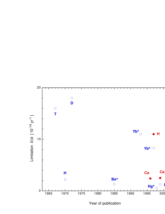
Figure 1: Strongest possible limits on the variation of the frequencies available in 2000. The limit is defined as a fractional uncertainty of the frequency divided by the time from the publication to 2000.

4 Some new options for precise comparison of frequencies

4.1 Hyperfine structure

For a while the hyperfine splitting of atomic levels has been a quantity available for the most precise measurements. Comparison of hfs in different atoms can give us precise information on the variation of the nuclear magnetic moment rather than on the fine structure constant.

• We start with the hydrogen hfs project. The hyperfine structure interval in the ground state of the hydrogen atom was frequently measured (see Sects. 6.1 and 6.2). For a preliminary estimation we accept a value

  $$\nu_{\sc hfs}({\rm H})=1420\,405.751\,766\,7(9)\;{\rm kHz}\,,$$ (22)

  which used to be presented in reviews (see e. g. Ref. [65]) as a final result for the hfs separation. The fractional uncertainty is about 6 parts in $10^{14}$ and on being divided by 30 years that gives $2\cdot 10^{-14}$ yr^-1. If the accuracy is now the same this should rather be multiplied by $\sqrt{2}$.

• Let us consider briefly a possible variation of the deuterium hyperfine separation, which was measured in 1972 [66] with an uncertainty of $5.2\cdot 10^{-12}$. The relative accuracy is much worse than for H (cf. Eq.(22)). However, the magnetic moment of a deutron (see Table 11) includes a large cancellation

  $$\mu({\rm D})\simeq\mu_{p}+\mu_{n}=|\mu_{p}|-|\mu_{n}|$$ (23)

  between the proton ($\mu_{p}=2.793\,\mu_{\sc n}$) and neutron ($\mu_{n}=-1.913\,\mu_{\sc n}$) contributions and this hfs value might be very sensitive to the variation of effective parameters of the strong interactions.

• The hfs of the ground state in the ¹⁷¹Yb⁺ ion can also provide a limit for the variation per year on a level of a few units in $10^{14}$. The most precise measurements are presented in Fig. 2, where the open circles are for preliminary results [84, 85], while the full ones are for final values [71, 72].

  

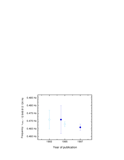
  Figure 2: Precise study of the hfs interval in the ground state of ${}^{171}Yb$.

  The disadvantages (in comparison to the hydrogen case) are: a less strong limit for the variation with less reliability (the result was reached with a high accuracy in two laboratories, but the precision was different by a factor 3).

• Generally, study of nuclei with small magnetic moments are expected to lead to sensitive tests for possible variations of the proton or neutron magnetic moment. We give a list of stable nuclei with small magnetic moments in Table 7. The tungsten ${}^{183}_{~{}74}$W has a halftime of $1.1\cdot 10^{17}$ yr and we include it in the table.

  		Natural	Nuclear	Magnetic
  $Z$	Isotope	abundance	spin and	moment
  			parity	[$\mu_{\sc n}$]
  7	15N	0.37 %	$1/2^{-}$	-0.283 188 4(5)
  19	41K	6.7 %	$3/2^{+}$	0.214 870 1(2)
  26	57Fe	2.2 %	$1/2^{-}$	0.090 44(7)
  39	89Y	100 %	$1/2^{-}$	-0.137 415 4(4)
  45	103Rh	100 %	$1/2^{-}$	-0.088 40(2)
  47	107Ag	52 %	$1/2^{-}$	-0.113 57(2)
  	109Ag	48 %	$1/2^{-}$	-0.130 56(2)
  64	155Gd	15 %	$3/2^{-}$	-0.259 1(5)
  	157Gd	16 %	$3/2^{-}$	-0.339 8(7)
  69	169Tm	100 %	$1/2^{+}$	-0.231 6(15)
  74	183W	14 %	$1/2^{-}$	0.117 784 76(9)
  76	187Os	1.6 %	$1/2^{-}$	0.064 651 89(6)
  77	191Ir	37 %	$3/2^{+}$	0.150 7(6)
  	193Ir	63 %	$3/2^{+}$	0.163 7(6)
  79	197Au	100 %	$3/2^{+}$	0.145 746(9)

  Table 7: Isotopes with small nuclear spin.

  Up to now, there is no way to measure the nuclear magnetic moment with an accuracy on the level $10^{11}$ or better. For nuclei with spin 1/2, our proposal is to measure the hfs of a neutral atom or ion and to search for a variation of that value. In the case of spin 3/2, a value of the hfs interval is essentially affected by the nuclear quadrupole moment. An exception is ⁴¹K, where the quadrupole term is also small and it is worthwhile studying the hfs. Fortunately, the stable nuclei with the smallest magnetic moments (namely, ⁵⁷Fe, ¹⁰³Rh and ¹⁸⁷Os) have spin 1/2 and we hope that the accurate study of the hfs of the nuclei with a small magnetic moment is possible.

  The nuclear magnetic moment of radionuclides can be even smaller, for example, for ${}^{198}_{~{}81}$Tl ($|\mu|<10^{-3}\,\mu_{\sc n}$, $I=2^{-}$, $T_{1/2}=5.3(5)$ h), ${}^{153}_{~{}62}$Sm ($\mu=-0.022\,\mu_{\sc n}$, $I=3/2^{-}$, $T_{1/2}=46$ h) and ${}^{192}_{~{}79}$Au ($\mu=-0.009(2)\,\mu_{\sc n}$, $I=1^{-}$, $T_{1/2}=4.9$ h). Our proposal for such isotopes is to measure a value of the shielded magnetic moment of the nucleus, investigating ions with coupled electrons only (Hg-, Os-, W-, Hf-, Ba-, Xe-like etc). Particularly, Hg-, Ba- and Xe-like ions have complete subshells and this is an advantage for the study of ¹⁹⁸Tl. We hope that a method developed in Ref. [86] to study a bound electron $g$-factor in H-like ions can be applied here. By achieving an uncertainty of about $10^{-9}$ for the magnetic moment, the limit for the variation of $g_{p}$ is expected to be on the level of $3\cdot 10^{-13}$ yr^-1. We should mention that not all magnetic moments of radionuclides with a halftime longer than 10 days are known [28] and it might happen, that some of them are even smaller than $10^{-3}\,\mu_{\sc n}$.

4.2 Fine structure

When the fine structure (proportional to $\alpha^{2}Ry$) is determined, it can be compared with the gross structure (proportional to $Ry$) and thus yielding a direct limit for a variation of the fine structure constant $\alpha$. The gross structure can be taken from measurements with neutral hydrogen and calcium atoms, and with strontium and indium ions and, maybe, in the future with other atoms.

• To date there are no competitive results on the fs. The best result for the atomic fine structure has been reached for the Ba⁺ ion [87]

  $$\nu_{\rm fs}(^{138}{\rm Ba^{+}},\;5d{}^{2}D_{3/2}-5d{}^{2}D_{5/2})=24\,012\,048\,317.17(44)\,{\rm kHz}\,.$$ (24)

  Note that this is for the fs of excited states. We think that some higher accuracy can be achieved by studying the fine structure associated with the ground state. If the subshell with valence $p$-electrons (or $d$) is open, the lowest excited states are due to the fine structure. The frequency can lie in radio-frequency range and the lines are very narrow. That is because of two reason: the $E1$ transition is not allowed for $P-P$ transitions and the decay rate is proportional to some power of the low transition frequency. Thus the lowest levels are split due to relativistic effects only and they can be measured accurately. This is another way of measuring the fine structure precisely. In combination with the gross structure, one can reach a limit for $\alpha$. The interpretation of such a comparison is simpler than in the case of hfs. A similar way is to study the relativistic correction for the gross structure is of use for astrophysical data [36]. In Table 8 we give a list of the rf transition of the low-lying fine structure in some neutral atoms, while those for different ions are collected in Table 9.

  $Z$	Atom	Level	Energy	Lifetime	Nuclear spin
  5	B(22P${}_{1/2}^{0}$)	22P${}_{3/2}^{0}$	0.457 THz	$3.2\cdot 10^{7}$ s	3 (10B), 3/2 (11B)
  6	C(23P0)	23P1	0.492 THz	$1.3\cdot 10^{7}$ s	0 (12C), 1/2 (13C)
  		23P2	1.30  THz	$3.7\cdot 10^{6}$ s
  14	Si(33P0)	33P1	2.31  THz	$1\cdot 10^{5}$ s	0 (28Si, 30Si), 1/2 (29Si)

  Table 8: Low-lying rf fine structure of neutral atoms.

  $Z$	Atom	Level	Energy	Nuclear spin
  6	C+(22P${}_{1/2}^{0}$)	22P${}_{3/2}^{0}$	1.90 THz	0 (12C), 1/2 (13C)
  7	N+(23P0)	23P1	1.46 THz	1 (14N), 1/2 (15N)
  		23P2	3.92 THz
  21	Sc+(3d4s$-{}^{3}$D1)	3d4s$-{}^{3}$D2	2.03 THz	7/2 (21Sc)
  		3d4s$-{}^{3}$D3	5.33 THz
  22	Ti+(3d24s$-{}^{4}$F3/2)	3$d^{2}(^{3}$F)4s$-{}^{4}$F5/2	2.82 THz	0 (46Ti, 48Ti, 50Ti),
  		3d24s$-{}^{4}$F7/2	6.77 THz	5/2 (47Ti), 7/2 (49Ti)
  23	V+(3d${}^{4}-{}^{5}$D0)	3d${}^{4}-{}^{5}$D1	1.08 THz	6 (50V), 7/2 (51V)
  		3d${}^{4}-{}^{5}$D2	3.20 THz
  		3d${}^{4}-{}^{5}$D3	6.26 THz
  		3d${}^{4}-{}^{5}$D4	10.17 THz

  Table 9: Low-lying rf fine structure of single-charged ions.

  Unfortunately, there are no systems in the tables which can be easily studied. In the case of neutral atoms in Table 8, laser cooling is hard to apply because of the metastable fine structure levels. Finding levels which are insensitive to the magnetic field is a problem for ions. These are (2³P₀) in N⁺ and (3d${}^{4}-{}^{5}$D₀) in V⁺. Finding proper means of detection of the fs transition can be another problem for a few-ions trap experiments.

• It is also possible to find an optical or infrared transition for the low-lying fine structure. Let us mention a transition

  $$\nu_{\sc fs}({\rm Pb},6{}^{3}P_{0}-6{}^{3}P_{2})\simeq 1.32~{}{\rm eV}$$ (25)

  in neutral lead, which can be studied by means of two-photon Doppler-free spectroscopy (the wave length of each photon is 1.88 $\mu$m). The excited level ${}^{3}P_{2}$ lives for 2.6 s and it is narrow enough to reach an accurate result. It has to be mentioned that in the case of neutral lead, calculations using $jj$ coupling are competitive with those using $LS$ one. Actually, a clear separation of non-relativistic and relativistic physics is only possible for $LS$ coupling. $LS$ coupling means that one must first find a non-relativistic energy level with $n^{*}(L)$ and next to take into account the (relativistic) spin effects. For $jj$ coupling the (relativistic) spin effects for individual electrons are more important than a (non-relativistic) interaction of their orbital momenta. We expect large relativistic corrections to the fine structure.

  

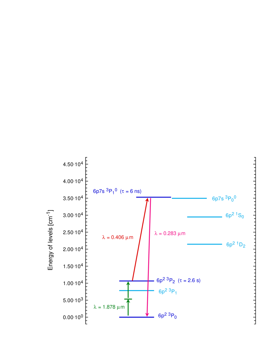
  Figure 3: The energy levels and a scheme of the experiment on the fine structure of neutral lead.

  One possible experiment is presented in Fig. 3. The ground state ($6p^{2}{\,}^{3\!}P_{0}$) of one of the spinless isotopes of lead (²⁰⁴Pb, natural abundance 1.4%; ²⁰⁶Pb, 24%; or ²⁰⁸Pb, 52%) is excited by two photons ($\lambda=1.878\,\mu m$) to a metastable ${}^{3}P_{2}$ level with a lifetime of 2.6 s. The line is narrow because of the metastability and of Doppler-free excitation. Detection of the ${}^{3}P_{2}$ level can be done using an additional one-photon excitation ($\lambda=0.283\,\mu m$) to a $6p7s{}^{3}P_{0}$ state and measuring the fluorenscence ($\lambda=0.406\,\mu m$).

• Alkali atoms have simple spectra and that is an advantage for both experiment [56, 77, 79, 87, 89] and theory [60, 53]. Measurement of the fine structure of such a system as a test for the variations of $\alpha$ was proposed by Jungmann [88] (cf. Ref. [36]) particularly for Ca⁺ and Sr⁺ ions. Similar measurement can be performed for In⁺. All these atoms are now a subject of some investigations as a part of efforts to design new optical standards. Let us discuss shortly the indium case. An accurate result for the fine structure may be obtained by considering the $5s5p-{}^{3}P_{J}$ levels in the ¹¹⁵In⁺ ion. The fs interval of excited levels cannot usually be measured precisely. For an indium ion it may however be determined as the difference between two gross transitions ($5s^{2}\!-\!{}^{1}S_{0}-5s5p\!-\!{}^{3}P_{J}$)ith different $J$. Indeed, since the fs interval is about 1% of the transition frequency for the gross structure, one can expect that the fractional accuracy is not very high. The advantage is that in the case of very accurate measurements of $5s^{2}\!-\!{}^{1}S_{0}-5s5p\!-\!{}^{3}P_{0}$ for different $P_{J}$-states, it may be possible to go beyond the accuracy of standards. As an example, let us recall the results on the $1s-2s$ transition in the hydrogen atom [75] and on the hydrogen-deuterium isotopic shift of the $1s-2s$ frequency [91]. By comparing the two frequencies, it was possible to detect a drift of the standard used and to reduce the absolute uncertainty to 150 Hz for the isotopic shift, while for hydrogen this was 850 Hz. The absolute measurement in the indium ion ($5S-5P_{0}$ transition) now gives [89] 1 267 402 452 914(41) kHz (uncertainty is $3.2\cdot 10^{-11}$) and the result is soon to be improved.

• Another approach to compare the gross and fine structure may possibly be realized in an atomic system, where the levels with different $n$ and $l$ lie close each to other. This may be in the case of an accidental cancellation of the $Ry$ and $\alpha^{2}Ry$ terms. An example of such a cancellation can be seen in the spectrum of the Ag atom. Two excited multiplets, $4d^{10}5p$ and $4d^{9}5s^{2}$ (one of the $4d^{9}5s^{2}$ lines is quite narrow $\sim 1$ Hz), are split slightly. The splitting comes from the gross structure. However, it is comparable with the internal structure of the multiplets, which is due to the relativistic corrections (fine structure). For such a cancellation, a value of energy splitting between levels from different multiplets is quite sensitive to a variation of $\alpha$. Measuring the splitting with relatively low accuracy, it is possible to reach a strong limit. A similar idea for the $4f^{10}5d6s-4f^{9}5d^{2}6s$ lines in the $Dy$ atom was proposed in Ref. [52, 53]. In some sense, the search for the accidental degeneration is quite close to approaches using nuclear data, in which the smallness of some differences is widely utilized (see e. g. Ref. [25]).

  Let us discuss conditions needed for success in such an experiment. We consider the spectrum of the Ag atom as an example and some properties of low-lying levels in that atom are presented in Fig. 4 and Table 10.

  

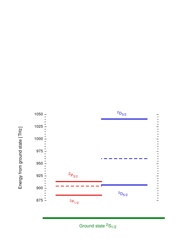
  Figure 4: Scheme of low-lying levels of the neutral Ag atom. The hyperfine structure is not shown.

  Ground state: $4d^{10}5s\;{}^{2}S_{1/2}$
  Excited states
  Level	Energy	Lifetime
  $4d^{10}5p\;{}^{2}P^{0}_{1/2}$	885.94 THz	$8\cdot 10^{-9}$ s
  $4d^{9}5s^{2}\;{}^{2}D_{5/2}$	906.64 THz	0.2 s
  $4d^{10}5p\;{}^{2}P^{0}_{3/2}$	913.55 THz	$7\cdot 10^{-9}$ s
  $4d^{9}5s^{2}\;{}^{2}D_{3/2}$	1040.70 THz	$9\cdot 10^{-5}$ s
  Fine structure
  Multiplet	The fs	Center of
  	splitting	gravity
  $4d^{10}5p\;{}^{2}P^{0}_{j}$	27.60 THz	904.35 THz
  $4d^{9}5s^{2}\;{}^{2}D_{j}$	134.06 THz	960.24 THz

  Table 10: Properties of low-lying excited states of the neutral silver atom. The hfs is neglected.

  The conditions for a precise measurement of a transition sensitive to possible variations of the constants are:

  • The fine structure terms should be of the same order of magnitude as the gross structure contributions. In the silver ion this is true: the splitting of the two $5p{}^{2}P^{0}_{J}$ levels is about the same value as the separation between one of them ($5p{}^{2}P^{0}_{3/2}$) and one of the $4d^{9}5s^{2}{}^{2}D_{J}$ levels ($4d^{9}5s^{2}{}^{2}D_{5/2}$). The other fine structure splitting (between $D$ levels) is larger than the $P-D$ interval.

  • The non-relativistic ($Ry$) and relativistic terms $\alpha^{2}Ry$ have to have a different sign. This is very likely because of the sandwich sequence of levels $P-D-P-D$ with the center of gravity of the $D$ level lying above that for the $P$ states. That means that the non-relativistic contribution for the $D$ states is likely higher than for the $P$ states. As far as we are interested in the lower $D$ level, we can expect that the relativistic contribution to that is negative. Indeed, if silver qualified for other conditions it would be studied theoretically before performing the experiment. The relativistic effects shift and split levels. We can estimate an enhancement of the sensitivity assuming that there are no shifts, but only splittings. We expect this should work for a preliminary estimation. In such a case a non-relativistic correction can be found from the separation of the centers of gravitation of the $P$ and $D$ lines:

    $$\Delta_{\rm NR}({}^{2}P^{0}_{1/2}-{}^{2}D_{5/2})=-55.89~{}{\rm THz}=A\,Ry\,,$$ (26)

    while the relativistic corrections are obtained from the shift of the energy level from the position of the center of gravity

    $$\Delta_{\rm Rel}({}^{2}P^{0}_{3/2}-{}^{2}D_{5/2})=62.82~{}{\rm THz}=B\,\alpha^{2}\,Ry\,.$$ (27)

    The separation eventually is equal to

    $$\Delta({}^{2}P^{0}_{3/2}-{}^{2}D_{5/2})=62.82~{}{\rm THz}-55.89~{}{\rm THz}=6.93~{}{\rm THz}\,.$$ (28)

    A variation of the Rydberg constant can be neglected and one can find

    $$\frac{\partial\ln(\Delta/Ry)}{\partial\ln\alpha}\simeq 2\,\frac{B\,\alpha^{2}Ry}{\Delta}\approx 2\cdot 10\,.$$ (29)

    The factor 2 is the common factor because any relativistic correction depends on $\alpha^{2}$ and 10 is an estimation of the enhancement due to the accidental degenerations.

  • For accurate measurement it may be important to use laser cooling. An important conditions for this is lack of the hyperfine structure. Unfortunately both stable isotopes (¹⁰⁷Ag and ¹⁰⁹Ag) have some magnetic moment and the ground state of any stable isotope is usually split into two states. The laser cooling is possible but rather complicated.

  • It may also be important to apply two-photon Doppler-free excitation to produce one of the two levels, splitting of which contains a cancellation between relativistic and non-relativistic term. This is necessary because it is somehow possible to cool the ground state, but not excited states. We have to eliminate Doppler effects due to excitation. The $D$ states in the silver atom can be excited by means of the two-photon transitions.

  • Both levels have to be narrow. The $D$ level ($4d^{9}5s^{2}{}^{2}D_{5/2}$) is very narrow with a width of about 1 Hz, but both $P$ states are very broad.

  • A precise measurement of the small splitting due to the cancellation must be possible. Generally this means that one must be to induce a single-photon transition. The one-photon transition between states $4d^{9}5s^{2}{}^{2}D_{5/2}$ and $5p{}^{2}P^{0}_{3/2}$ lies at 7 THz. It can be induced but it is hard to measure such a transition frequency precisely.

  One can see that the conditions can be realized in some atomic systems and it is necessary to search for them. One should note that in the case of ions the condition for choice of nuclear spin is different. It may be more important to have some states that are insensitive to a magnetic field (the whole moment $F$ of a system of electrons plus nucleus must be integer and states with $m_{F}=0$ are alowed).

  Our suggestion is to look for a relatively small enhancement but with an appropriate possibility for precise measurements. The proposal with $Dy$ in Refs. [52, 53] is rather for a great enhancement without any accurate spectroscopy.

5 Nuclear magnetic moments and interpretation of the frequency comparisons

A frequency comparison involves atoms that are very differentin nature and one must be prepared to interpret results. Most precise results are for the hfs (see Table 5) and we mainly discuss the hfs transitions. Since any absolute measurements assume a comparison to the cesium hyperfine separation this is also important for interpreting the absolute optical measurements (see Table 6).

5.1 Magnetic moments

To the leading order the hfs interval can be presented in the form of Eq.(2). There are two different factors important for the comparison: magnetic moments and the relativistic corrections. The magnetic moments and some other nuclear properties are collected in Table 11. Some atoms, hyperfine separation in which was measured accurately, but less precisely than one part in $10^{11}$, are also included:

• $\nu_{\sc hfs}({}^{43}{\rm Ca}^{+})=15\,199\,862.858(2)$ kHz [92];

• $\nu_{\sc hfs}({}^{113}{\rm Cd}^{+})=3\,225\,608.286\,4(3)$ kHz [93];

• $\nu_{\sc hfs}({}^{131}{\rm Ba}^{+})=9\,107\,913.699\,0(5)$ kHz [70];

• $\nu_{\sc hfs}({}^{135}{\rm Ba}^{+})=7\,183\,340.234\,9(6)$ kHz [94];

• $\nu_{\sc hfs}({}^{137}{\rm Ba}^{+})=8\,037\,741.667\,7(4)$ kHz [95].

Most of these are stable, expect cadmium ($T_{1/2}({}^{113}{\rm Cd})=9\cdot 10^{15}$ yr) and the lightest barium ($T_{1/2}({}^{131}{\rm Ba})=12$ d). The sign of the magnetic moment of ¹³¹Ba was presented in Ref. [28] as unknown and we follow Ref. [70].

A discussion on the value of the nuclear magnetic moments is also important because of our proposal to look for variations of small moments.

		Nuclear	Magnetic
$Z$	Nucleus	spin and	moment
		parity	[$\mu_{\sc n}$]
	H	1/2+	2.793
	D	1+	0.857
	T	1/2+	2.979
4	9Be	3/2-	-1.178
20	43Ca	7/2-	-1.318
37	87Rb	3/2-	2.751
48	113Cd	1/2+	-0.622
55	133Cs	7/2+	2.582
56	131Ba	1/2+	-0.708
	133Ba	1/2+	-0.772
	135Ba	3/2+	0.838
	137Ba	3/2+	0.938
70	171Yb	1/2-	0.494
	173Yb	5/2-	-0.680
80	199Hg	1/2-	0.506

Table 11: Properties of some nuclei important for precise microwave spectroscopy.

All nuclei in Table 11 and 7 have an odd value of $A$, while $Z$ is even for iron, gadolinium, osmium and tungsten (Table 7) and calcium, cadmium, barium, ytterbium and mercury (Table 11) and odd for all others. An even value of $Z$ indicates that the nuclear magnetic moment is associated with the neutron magnetic moment and in the case of odd $Z$ the moment is due to the proton one. Let us start with small moments. Some of these can be understood using a simple model (the Schmidt model), while assuming that the magnetic moment of the nucleus—like a moment of an electron in a hydrogen-like atom—includes a spin part and an orbital part

$$\mbox{\boldmath{$\mu$}}_{a}(I)=\mu\,{\bf I}/{I}=\mu_{a}^{s}{\bf S}+\mu_{a}^{l}{\bf L}\,,$$ (30)

where ${\bf I}={\bf S}+{\bf L}$, $\mu_{p}^{s}=2\mu_{p}$, $\mu_{n}^{s}=2\mu_{n}$, $\mu_{p}^{l}=\mu_{\sc n}$ and $\mu_{n}^{l}=0$. We should remember that the values of the spin terms ($\mu_{a}^{s}$) originate from dynamic effects of Quantum Chromodynamics (QCD) in the strong coupling regime and so they sensitive to a variation of the QCD coupling constant ($\alpha_{\sc s}$). The Schmidt model leads to some relatively small values in a few cases:

• for odd $Z$, $I=1/2$, $L=1$, in particular, N, Y, Rh and Ag in Table 7 (a cancellation between spin and orbit contributions)

  $$\mu=\frac{4-g_{p}}{6}\,\mu_{\sc n}\sim-0.26\,\mu_{\sc n}\,,$$ (31)

  where $g_{p}=2\cdot 2.793\dots$;

• for odd $Z$, $I=3/2$, $L=2$, particularly, K, Ir and Au in Table 7 (a cancellation between spin and orbit contributions):

  $$\mu=\frac{3}{10}\,\Big{(}6-g_{p}\Big{)}\,\mu_{\sc n}\sim 0.12\,\mu_{\sc n}\,;$$ (32)

• for even $Z$, $I=1/2$, $L=1$, in particular, iron, osmium and tungsten in Table 7, ytterbium–171 and mercury in Table 11 and ${}^{153}_{~{}62}$Sm, discussed in Sect. 4.1 (the result is relatively small because of the coefficient 1/3):

  $$\mu=-\frac{g_{n}}{6}\,\mu_{\sc n}\sim 0.64\,\mu_{\sc n}\,,$$ (33)

  where $g_{n}=-2\cdot 1.913\dots$.

In all other cases presented in Tables 11 and 7 the value of the magnetic moment is not smaller than one in units of the nuclear magneton $\mu_{\sc n}$. In some cases the agreement between the Schmidt values and the actual ones is a 10% level, but in other cases the actual values are significantly smaller and that is a result of the nuclear effects and, hence, small magnetic moments are sensitive to these. Comparison of Eqs.(31), (32) and (33) shows that the nuclei with odd $Z$ and odd $A$ can be more interesting because the magnetic moment is small partly due to cancellations between the spin and orbit contributions, which are sensitive to variation of $g_{p}$.

We collect the Schmidt values for different nuclear spin

$$\mu_{\sc s}(I=L\pm 1/2)=I\,\left(g^{l}\pm\frac{g^{s}-g^{l}}{2l+1}\right)\mu_{\sc n}\,,$$ (34)

where $g^{b}=\mu^{b}/\mu_{\sc n}$ and $\mu^{b}$ for a proton and neutron are defined above, in Table 12.

	Spin ($I$) and Schmidt value of the magnetic moment ($\mu_{S}$) of odd-$A$ nuclei
$l$	$I=l+1/2$			$I=l-1/2$
	$I$	Magnetic moment [$\mu_{\sc n}$]		$I$	Magnetic moment [$\mu_{\sc n}$]
		Odd $Z$	Even $Z$		Odd $Z$	Even $Z$
0	1/2+	$g_{p}/2~{}~{}~{}~{}~{}\simeq 2.793$	$g_{n}/2\simeq-1.913$	-	-	-
1	3/2-	$g_{p}/2+1\simeq 3.793$	$g_{n}/2\simeq-1.913$	1/2-	$1/3\,\big{(}2-g_{p}/2\big{)}\simeq-0.264$	$1/3\,\big{(}-g_{n}/2\big{)}\simeq 0.638$
2	5/2+	$g_{p}/2+2\simeq 4.793$	$g_{n}/2\simeq-1.913$	3/2+	$3/5\,\big{(}3-g_{p}/2\big{)}\simeq~{}0.124$	$3/5\,\big{(}-g_{n}/2\big{)}\simeq 1.148$
3	7/2-	$g_{p}/2+3\simeq 5.793$	$g_{n}/2\simeq-1.913$	5/2-	$5/7\,\big{(}4-g_{p}/2\big{)}\simeq~{}0.862$	$5/7\,\big{(}-g_{n}/2\big{)}\simeq 1.366$
4	9/2+	$g_{p}/2+4\simeq 6.793$	$g_{n}/2\simeq-1.913$	7/2+	$7/9\,\big{(}5-g_{p}/2\big{)}\simeq~{}1.717$	$7/9\,\big{(}-g_{n}/2\big{)}\simeq 1.488$

Table 12: Magnetic moment, spin and parity of nuclei in the Schmidt model (Eqs.(30) and (34)).

Comparison of the Schmidt model with the most important isotopes for precision measurements and variations of the constants is presented in Fig. 5. Here we collect the Schmidt values (two lines) and actual values of the magnetic moments of the isotopes from Table 11 (filled circles), other stable or long-lived isotopes associated with simple atomic spectra of neutral or single-charged ions (open circles), and the isotopes from Table 7 with small magnetic moments (triangles). One nucleus of this kind (⁸⁷Sr, 9/2⁺, $\mu=-1.094\mu_{\sc n}$, $\mu_{\sc s}(9/2^{+})=-1.931\mu_{\sc n}$)) is not included in the figure because of its large spin.

From the figure one sees that the agreement between real values and the simple Schmidt model is not perfect. This means that nature of nuclear spin are more complicated and the effects of nuclear interaction are significant. However, the model contains some important physics: e. g. the model predicts simple relations between the nuclear parity and magnetic moment. Only one isotope in Fig. 5 has inconsistent values of the parity and spin (¹⁶⁹Tm, 1/2⁺, $\mu=-0.23\mu_{\sc n}$).

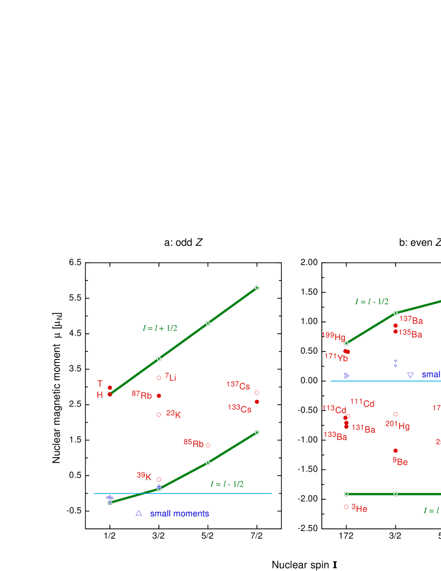
Figure 5: Magnetic moment of some isotopes: actual values and the Schmidt model. Nuclei with small magnetic moments are listed in Table 7.

There is no simple model for even $A$, when there are two valence particles—a proton and neutron—and a contribution of orbital motion. For deuterium the proton and neutron contributions have different signs (23). Two radionuclides discussed in Sect. 4.1, ${}^{198}_{~{}81}$Tl, ${}^{192}_{~{}79}$Au, have even $A$.

5.2 Relativistic corrections

Now let us discuss the hfs intervals in Table 5. First, we consider the relativistic corrections, which have been in part discussed in Sect 3.2. They can be calculated within using many-body perturbation theory (see e. g. Ref. [53]). An approximation of Eqs.(18) and (19) is a good one for alkali atoms (all but ytterbium and mercury in Table 5) under the conditions:

• High nuclear charge: $Z\gg 1$.

• Atoms are neutral or slightly charged: $Z\gg z$, where $z$ is an effective charge of a compound nucleus for the valentce electron, i. e. $z=1$ for neutral atoms and $z=2$ for single-charged ones. Note that, Eq.(18) is incorrect for hydrogen and its isotopes and for the Li-like ion of beryllium presented in Table 5.

• Accuracy is expected to be on a $5-15\%$ level and a comparison of two atoms with a small charge difference ($Z_{1,2}\gg|Z_{1}-Z_{2}|$) will not give accurate results.

As already mentioned, due to a discussion on the interpretation of results in Ref. [58], any atom with a closed subshell and one valence electron satisfies the above conditions. Alkali atoms actually form only one example of such atomic systems.

Relativistic corrections are also important for the gross and fine structure. They have a relative order of $(Z\alpha)^{2}$. In the simplest case, namely for alkali atoms, they were discussed in Ref. [53], where some results were obtained for Ca and Sr⁺ and in Ref. [96] for In⁺. It seems that relativistic effects are less important for the optical transitions than for the hfs because of relatively small numerical coefficients and an extra $1/n^{*}$ factor.

In the hydrogen atom for both hfs and $1s-2s$ transitions the corrections are negligible.

5.3 Hyperfine structure

The hfs of atoms with nuclei with even $Z$ and odd $A$ is sensitive to the neutron magnetic moment. In particular the Schmidt model predicts the magnetic moment of mercury and ytterbium–171 (see Eq.(33)) within 15% uncertainty. In contrast the hfs of atoms with odd $Z$ and odd $A$ depends on a value of the proton magnetic moment. An important point however is the size of nuclear effects of the strong and electromagnetic interactions. They can be estimated by a deviation from the Schmidt value. In the case of Cs the nuclear effects increase the value by a factor of about 1.5. This means that any interpretation of comparisons with Cs cannot neglect the strong interactions.

In the case of even-to-even or odd-to-odd comparisons, in particular for H–Rb, and Be–Yb–Hg, we expect an information on the variation of the constants due to the nuclear effects and the relativistic corrections. Comparison of odd-to-even hfs yields to variation of $g_{n}$ with respect to $g_{p}$. This is important, because there is no reason to expect that a value of $g_{n}/g_{p}$ is relatively stable, while the constants are varying. Our point of view is different from that in Ref. [58], where the H–Hg⁺ comparison was examined assuming that a variation of the nuclear $g$-factors can be neglected.

We have not mentioned the Cs hfs because here the interpretation is slightly different. Although ¹³³Cs is an isotope with odd $Z$, its comparison with H or Rb is sensitive to a variation of $g_{p}$, because the $g_{p}$ contribution to the nuclear $g$ factor has a negative sign in contrast to H and $Rb$. For example, the sensitivity of the H-to-Cs comparison to the $g_{p}$ variation is determined by the value of

$$\frac{\partial}{\partial\ln{g_{p}}}\,\ln\frac{\mu_{\sc s}({\rm Cs})}{\mu_{\sc s}({\rm H})}=-\frac{10}{10-g_{p}}\simeq-2.3\,,$$ (35)

and for the Rb-to-Cs comparison one can find

$$\frac{\partial}{\partial\ln{g_{p}}}\,\ln\frac{\mu_{\sc s}({\rm Cs})}{\mu_{\sc s}({\rm Rb})}=-\frac{12\,g_{p}}{\big{(}2+g_{p}\big{)}\,\big{(}10-g_{p}\big{)}}\simeq-2.0\,.$$ (36)

In contrast, the H-to-Rb comparison is actually insensitive to any variations of the proton $g$-factor:

$$\frac{\partial}{\partial\ln{g_{p}}}\,\ln\frac{\mu_{\sc s}({\rm Rb})}{\mu_{\sc s}({\rm H})}=-\frac{2}{2+g_{p}}\simeq-0.26\,.$$ (37)

	Magnetic moment				Relativistic
Atom	Naive ($\mu_{\sc s}$)		Actual ($\mu$)		correction
	Eq. for $\mu_{\sc s}$ [$\mu_{\sc n}$]	[$\mu_{\sc n}$]	[$\mu_{\sc n}$]	$\mu/\mu_{\sc s}$	$F(\alpha)$	$\partial\ln F/\partial\ln\alpha$
H	$g_{p}/2$	2.79	2.79	1.00	1.00	0.00
D	$(g_{p}-|g_{n}|)/2$	0.88	0.86	0.98	1.00	0.00
9Be+	$g_{n}/2$	-1.18	-1.91	0.62	1.00	0.00
87Rb	$g_{p}/2+1$	3.73	2.75	0.74	1.15(10)	0.30(6)
133Cs	$\frac{7}{18}(10-g_{p})$	1.72	2.58	1.50	1.39(7)	0.83, [53]
171Yb+	$-g_{n}/6$	0.64	0.49	0.77	1.78 (9)	1.42(15)
199Hg+	$-g_{n}/6$	0.64	0.51	0.80	2.26(12)	2.30, [53]

Table 13: Hyperfine structure properties. Relativistic corrections, if not specified, are calculated from Eqs.(18) and (19). We estimate the uncertainty for $F$ as 5% and for the derivative as 10% by comparison with Ref. [53]. In the case of hydrogen and beryllium, the Casimir correction is not appropriate, but Eqs.(15), (16) and (17) lead to negligible shifts.

We summarize some properties of hfs intervals of some atoms in Table 13. The naive value ($\mu_{\sc s}$) is the Schmidt one ((see Table 12) for any atom, except deuterium. The deuterium naive value is determined from Eq.(23). It is not quite clear if the Schmidt model works, but we expect it to be appropriate for preliminary estimations and we consider deviations from the naive value $\mu/\mu_{\sc s}-1$ as a correction due to nuclear interactions. For Cs, the corrections shift the value by 50% and unsurprisingly that is the largest contribution in Table 13. Cesium has only one stable isotope and this indicates that the nuclear configuration is not strongly bounded and so different nuclear core polarization effects or an admixture of excited states can be significant. We have included the beryllium ion in the Table mainly due to the measurement [82] in the magnetic field. In the leading non-relativistic approximation this value is proportional to the hfs interval at zero field. The relativistic corrections are different, but they are small enough.

Relativistic corrections are calculated using Casimir approach of Eqs.(18) and (19), except for derivatives for Cs and Hg, taken from Ref. [53]. One reason, why derivatives are relatively large is that the function $F$ is always a function of $\alpha^{2}$. However, one can expect the same for the strong interactions. One can see that the relativistic corrections for alkali atoms are of the same sign and it must be a partial cancellation for the comparison of two different hfs. In contrast, the nuclear effects shift a value of the nuclear magnetic moment in different directions for different atoms and an enhancement (e. g. for the Rb–Cs hfs) is possible. We can however hope that for a representative enough set of atoms they can be considered rather as statistical errors.

Clearly if we would like to have a clear interpretation of some frequency comparisons, we have to choose one of two options:

• We can measure only the gross and fine structure with understandable relativistic effects and reach a limit for the variation of $\alpha$.

• We can involve the hfs in the comparison. In this case we must be able to estimate nuclear effects and their variations. The magnetic moment can be close to the Schmidt value accidently due to some cancellation of contributions with different nature and it can be quite sensitive to the variations of the constants. So it is necessary to have small and understandable corrections due to the nuclear effects. It is also necessary to do a few comparisons in order to be able to transform variations of the frequencies to variations of $\alpha$, $g_{p}$, $g_{n}$ and $\mu_{\sc n}/\mu_{\sc b}$. One should emphasize a significant difference between the study of atoms with odd $A$ and either odd or even $Z$. The even $Z$ nuclear magnetic moments are mainly proportional to the same value ($g_{n}$), which can be corrected by nuclear effects. A comparison between two even $Z$ hfs is insensitive to any variations $g_{n}$. Conversely investigation of only odd $Z$ atoms should provide enough information on $g_{p}$ because they contain spin and orbit contributions which diferently depend on nuclear quantum numbers ($L$, $S$ and $J$).

In principle, there is one more option search available. One can look for two isotopes (with odd $Z$ and odd $A$, but different nuclear spins or parity) of one element with magnetic moments close to their Schmidt values. The ratio of the hfs intervals should be free off any relativistic and many-body atomic corrections and could be not too sensitive to nuclear effects. In this case the ratio of the hfs should be close to a ratio of their respective Schmidt values, i. e. a simple function of $g_{p}$. Unfortunately we have been not able to find an appropriate pair of the isotopes for this study.

5.4 Time structure of the measurements

We should point out a timing problem in the absolute frequency measurements. Some results have been obtained via a direct comparison to the primary cesium clock, i. e. directly compared to the Cs hfs. Others have been compared indirectly and the “time structure” of such an experiment can be quite complicated and includes some intermediate steps with comparisons between different secondary standards. An example is a measurement of the $2s-8s$ and $2s-8d$ transitions in hydrogen and deuterium atoms by the Paris group. The measurements [97] involved a comparison in 1997 of the hydrogen and deuterium lines with some secondary standard, gauged in 1985 [98]. The standard was recalibrated in 1999 [99]. Such a time structure is reasonable for a determination of the Rydberg constant and the hydrogen Lamb shift, but it is not appropriate to search for a variation of the constants. In Tables 5 and 6 we assume that publication time is the time for a direct comparison with a primary Cs standard. For the hydrogen and deuterium hyperfine structure that is approximately correct. In some cases that is not so.

The other time structure problem is in a comparison with secondary standards, like a hydrogen maser. Some preliminary studies estimated possible deviations of its frequency with respect to some known standards or with respect to some average value of an ensemble of masers. In both case it is not clear how to interpret any comparison with a specific maser at some particular time.

6 The hyperfine separation in the hydrogen atom

6.1 Historical remarks

The hydrogen hfs was studied for a few generations of experiments. The first results with an accuracy of about $10^{12}$ were reached about 35 years ago and some of them are presented in Table 14. Most experiments [100, 101, 102, 103] were devoted to a measurement of the maser frequency, while previously measured value for the wall-shift using another maser in Ref. [113] was accepted. In Ref. [102] no explicit value of uncertainty was claimed. From discussions in that paper we estimate it as $3\cdot 10^{-12}$ for the NRC cesium standard and $1.7\cdot 10^{-12}$ for the maser.

Frequency ($\nu$)	Ref. to	Year	Relative	Ref. to
[kHz]	frequency		uncertainty	wall-shift
1 420 405.751 786(2)	[100], 1966	1965	$1.4\cdot 10^{-12}$	[104]
1 420 405.751 756(3)	[101], 1968	1966	$2.1\cdot 10^{-12}$	[104]
1 420 405.751 758(2)	[101], 1969	1967	$1.4\cdot 10^{-12}$	[104]
1 420 405.751 776(5)	[102], 1968	1968	$3.5\cdot 10^{-12}$	[104]
1 420 405.751 777(3)	[103], 1970	1968	$2.1\cdot 10^{-12}$	[104]

Table 14: Some early precise measurements of the hydrogen hyperfine separation. The references are given with the year of publication, while the year of the experiment is given additionally.

One of the first really accurate experiments was performed by NBS [105] and in part by Harvard University team [106]. It was pointed out [105] that the wall-shift and the frequency have to be determined in the experiments for the same masers. This generation of experiments [107, 105, 106, 108, 109, 110, 111, 112, 113] is discussed in the next section. When we speak about two generations we refer to an ideology, rather than to a time-frame. Some other experiments [116, 117, 118, 119, 120, 121] performed in that time or slightly earlier were not so precise (see Fig. 6). Let us mention Ref. [116] wherein an experiment that measured both the frequency and the wall-shift was described. However, only two bulbs were used. As was noted in Ref. [105] another important condition for appropriate results is the use of a large number of bulbs of different size (e. g. in Ref. [105] 11 bulbs were and in Ref. [106] the number was 18).

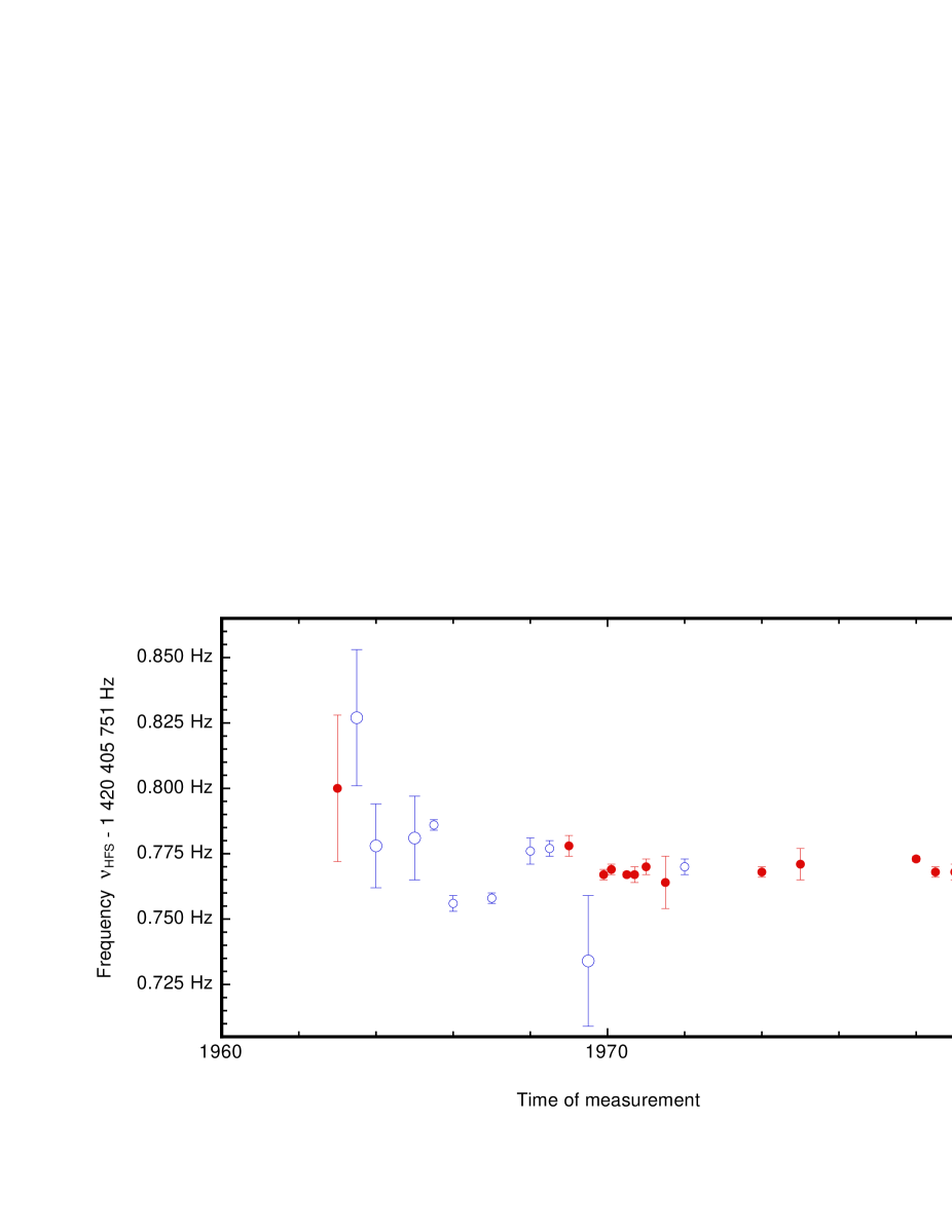
Figure 6: Precise experimental results on the hydrogen hyperfine separation. Filled circles are for those when the wall-shift was measured together with the frequency, while the open ones are for frequency measurements using a value of the wall-shift found separately for another maser.

6.2 Thirty years ago

About thirty years ago a number of precise results for the hfs interval in the ground state of the hydrogen atom were published [107, 105, 108, 109, 110, 111, 112, 113, 114, 115]. That was due to a trial to use the hydrogen maser as a primary frequency standard. The results are collected in Table 15. Until the publication of results Eq.(21) of experiment on the hfs of the beryllium ion fifteen years ago [82], the value of the hyperfine separation in the hydrogen atom had been the most precisely measured physical quantity.

#	Frequency ($\nu$)	Ref.	Year	Relative	Cs standard	Comment
	[kHz]			uncertainty
1	1 420 405.751 778(4)	[107], 1969	1969	$28\cdot 10^{-13}$	LSRH commerc.	2 bulbs
2	1 420 405.751 769(2)	[105], 1970	1969–1970	$14\cdot 10^{-13}$	NBS primary	Exp. 1, 12 bulbs [106]
3	1 420 405.751 767(2)	[105], 1970	1969–1970	$14\cdot 10^{-13}$	NBS primary	Exp. 2, 18 bulbs
4	1 420 405.751 768(2)	[105], 1970	1969–1970	$14\cdot 10^{-13}$	NBS primary	Exp. 1 & 2
5	1 420 405.751 767(1)	[108], 1971	1970	$7.0\cdot 10^{-13}$	NPL primary	6 bulbs
6	1 420 405.751 770(3)	[109], 1971	1970–1971	$21\cdot 10^{-13}$	NRC primary	5 bulbs
7	1 420 405.751 767(3)	[110], 1973	1970	$21\cdot 10^{-13}$	NPL primary	6 bulbs
8	1 420 405.751 768(2)	[111], 1974	1974	$14\cdot 10^{-13}$	LORAN C, USNO	Flexible bulb
9	1 420 405.751 770(3)	[112], 1974	1972	$21\cdot 10^{-13}$	TOP, TAF	Wall-shift [106]
10	1 420 405.751 771(6)	[113], 1978	1975–1976	$41\cdot 10^{-13}$	LORAN C	6 bulbs
11	1 420 405.751 768(2)	[114], 1980	1979	$14\cdot 10^{-13}$	LORAN C	5 bulbs
12	1 420 405.751 768(3)	[114], 1980	1979	$21\cdot 10^{-13}$	LORAN C	5 bulbs
13	1 420 405.751 773(1)	[115], 1980	1978	$~{}7\cdot 10^{-13}$	TAF	Flexible bulb,
						zero wall-shift

Table 15: The most precise measurements of the hydrogen hyperfine structure interval. The references are given with the year of publication, while the year of the experiment is given additionally. The abbreviations are: NBS—former National Bureau of Standards (USA), NPL—National Physical Laboratory (UK), NRC—National Research Council (Canada), LORAN C—a navigation system signal controlled by a cesium standard, USNO—U. S. Naval Observatory, TOP—cesium clock from the Paris Observatory, TAF—the French atomic time.

The experiments were performed using hydrogen masers and two key values were measured simultaneously: the frequency of the maser and the wall-shift. Result #9 is an exception: the authors utilized a value of the wall-shift from Ref. [106]. Result #5 of Ref. [108] with the smallest uncertainty was actually a preliminary presentation. The final value of the NPL experiment (result #5) had an accuracy [110] three times lower. One of the papers contains a report on two independent measurements [105], quoted as experiment 1 and experiment 2, and we give both results in the table, as well as an average value presented by the authors of Ref. [105]. Experiment 2 is a pure NBS experiment. In experiment 1 the maser frequency of a maser from Harvard university was measured with respect to the NBS primary cesium standard [105], while the wall-shift of the same maser was measured by the Harvard people [106]. The same result for the wall-shift [106] was accepted by the authors of Ref. [112] for another maser, the frequency of which they measured. Values #11 and #12 were presented in Ref. [114]. That paper is devoted to a measurement of the wall-shift and the unperturbed maser frequency (result #11) at the Shanghai Bureau of Metrology. It also contains a reference to an unpublished result (#12) for the unperturbed hydrogen frequency of two hydrogen maser by the Shaanxi Asrtonomical Observatory. In this two bulbs from the SBM were used. The last result in Table (# 13) is based on a different idea. Authors studied the temperature dependence of the wall-shift and they found the the shift vanished at some temperature $T_{0}$. The hfs interval was afterwards determined from a maser frequency at $T_{0}$.

The value in Table 5 (Eq.(22)) calculated by Ramsey [65] is an average of results #4 and #5, and so cannot be actually accepted. However, the results in Table 15 are consistent (apart from the earliest one) and one can calculate some average values. For instance the average values can be calculated over results ##1–3, 6–13 (a wide set) or over ##4, 6, 7, 10 and 11 (a conservative set). The wide set includes all original results, while the conservative one contains only values published in refereed journals. We consider results #1 and #7 as preliminary and also exclude result #8 because the wall-shift and the frequency werenot measured during the same experiment.

As a preliminary estimation, one can assume that the uncertainties are independent and one finds:

$$\nu_{\rm wide}=1\,420\,405.751\,770\,4(6)\;{\rm kHz}$$ (38)

and

$$\nu_{\rm cons}=1\,420\,405.751\,768\,3(12)\;{\rm kHz}\,.$$ (39)

The fractional uncertainty of the average value is (4–9)$\cdot 10^{-13}$ and that is approximately as in Table 5. In fact there has to be some correlation between the systematic errors. However since most of the results are consistent, any averaging cannot yield a value that is less precise than one of the results, namely

$$\nu(\#4)=1420\,405.751\,768(2)\;{\rm kHz}\,.$$ (40)

We think this result should be used for comparisons because it is the most accurate and reliable result in Table 15. Result #4 was published in a refereed journal [105] (in contrast to result #8 [111]) and it was based on two independent measurements of the unperturbated hydrogen hfs frequency with respect to the NBS primary Cs standard. The largest number of bulbs was used to determine the wall-shift using two independent experiments [106, 105]. The result is in fair agreement with other results in Table 15, apart from results #1 and # 13. The discrepancy with the former is not important, because result #1 does not agree with others on a one-sigma level, but rather within three sigma. We also should mention that Ref. [109] refers to a private communication by one of the authors of Ref. [107] (Menoud, 1971) wherein a new LSRH value of hydrogen hfs

$$\nu({\em LSRH})=1\,420\,405.751\,764(10)~{}{\rm kHz}\,,$$ (41)

is quoted. This is less precise than result #1 but agrees with other results. Two results in Table 15 are more precise than the value in Eq.(40). One of them (# 5) [108] was later corrected by the authors [110]. The other (result # 13) was obtained using very different methods. We do not include it in the conservative set since it is inconsistent with most other results of this set. To conclude, we present in Fig. 7 an overview of experiments done about 30 years ago. Most experimental results measured the wall-shift together with the frequency. Some details on the crucial results can be found in the Appendix.

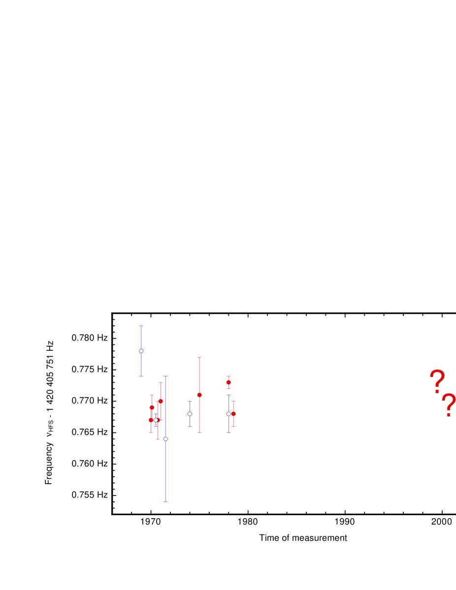
Figure 7: Hydrogen hyperfine structure as measured thirty years ago. Result with measurement of the wall-shift and the frequency for the same masers. Open circles are for preliminary results (conference proceedings, private communications) and results, corrected after publications. Full circles are for the final results. The question marks are for the possible 2000 measurements.

One should note that 30 years ago the accuracy of the primary cesium standards was not so high as now and this was an important source of uncertainty. The results in Table 15 are presented together with the name of the primary cesium standard used. We expect that it is possible to study variations of those standards which were frequently discussed due to international comparisons. We also expect that the reference set for comparison with experiments possible in the year 2000 will to be between the conservative and wide ones. Particularly, the main sources of uncertainty in experiments 1 and 2 in Ref. [105] are, in part, independent.

6.3 Why it is important to do experiment with hydrogen now

The hydrogen atom can now be used in the search for a limit for the variations of fundamental constants on a level that is comparable with most other possible projects. If the Paris group have really reached a level of accuracy ($\delta\nu/\nu\simeq 2.4\cdot 10^{-15}$) reported [122] as a preliminary result

$$\nu_{\sc hfs}({}^{87}{\rm Rb})=6\,834\,682.610\,904\,333(17)\;{\rm kHz}\,,$$ (42)

then only the work on the Rb clock and the Rb hfs can provide a significantly more precise test for the variations. Usually, it takes some time to really remove all sources of systematic errors after the first announcement of a performed measurement with a significantly better accuracy. The ratio of Rb and Cs hfs may also be less sensitive to the variations, and therefore it is not enough to compare two hfs transitions only. It is necessary to have several different data sets.

In any case, the study of the hydrogen hfs has a number of advantages, as are listed below:

• This is the only accurate comparison over a long interval (30 yr). Only the ¹⁷¹Yb⁺ hfs and the ⁹Be⁺ in the magnetic field (with a shorter time separation) is comparable to this. The other results obtained five or more years ago cannot provide a search for a variation of the constants on a level below $10^{-13}\,{\rm yr}^{-1}$.

• The result was obtained 30 years ago independently in a few different laboratories (see Table 15) after long studies over a number of years. Only ytterbium–171 was measured in two laboratories, whereas other transitions from Tables 5 and 6 have been studied in only one place for each atom.

• Most of the measurements of the hydrogen hfs were performed by direct comparisons with primary Cs clocks and thus they have simple time structures.

• Nowadays, this measurement can be also done in a number of laboratories.

• There is no direct problem due to the accuracy of any primary frequency standard because of the relatively low accuracy needed for the measurement.

• The measurement should be as precise as possible. If a level better than 10^-14 is achieved, a repetition in a few years can yield another strict limit for the variation of the constant. Thus the measurement in the year 2000 can be the “second” measurement of a 30-years test and the “first” measurement of a few-years test of the variation.

• Combining the variation of the H–Cs hfs with a variation of $1s-2s$ in the hydrogen atom with respect to the Cs hfs, one can achieve an estimation for a variation of the hydrogen hfs with respect to the Rydberg constant. The former limit is going to be about $(2-5)\cdot 10^{-14}$ yr^-1. The accuracy of a determination of the $1s-2s$ frequency in the hydrogen atom with respect to the Cs hfs has been improved and the uncertainty in 1999 [123] is about $6\cdot 10^{-14}$ yr^-1. This indirect comparison between the hfs and the $1s-2s$ frequency in hydrogen can be interpreted without any difficulties arising from the relativistic corrections or unclear nuclear effects. Only properties of fundamental particles are to be compared: $\alpha$ and $\mu_{p}/\mu_{\sc b}$.

The hydrogen experiment must have systematic errors, which are quite different from the short-term comparisons. The value of $\mu_{p}$ is on for the simplest for interpreting. The result can be reproduced in different laboratories. The expected limit for the variation of the hydrogen hfs lies between $2\cdot 10^{-14}$ yr^-1 and $5\cdot 10^{-14}$ yr^-1. This depends on the possibility of averaging the values from Table 15. Some additional analysis of the old data [107, 105, 109, 110, 111, 112, 106, 113] is needed. This would include the more recent data of international comparisons on the national primary standards utilized in the hydrogen experiments [107, 105, 109, 110, 111, 112, 113]. In 2000 only the Rb hfs can provide a significantly better result. From published values, we estimate the limits from possible experiments to approximately $1.3\cdot 10^{-14}$ yr^-1 (for Rb) and $1.1\cdot 10^{-14}$ yr^-1 (for Hg⁺). The latter is different from that presented in Table 5 because we expect significant correlations between the uncertainties of the original measurement and the repetition.

7 Conclusions

The strongest published limits (better than $10^{-16}$ yr^-1) on the variation of fundamental constants arise from geophysical data. However, any direct use of such estimations is not possible because of a incorrect interpretation of the data. The best astrophysical data gives limits between $10^{-14}$ and $10^{-15}$ yr^-1 and they are only slightly better than laboratory limits. Cosmological methods (such as investigation of nucleosynthesis and microwave background radiation) are far less precise, but they may be important if the variations at the beginning of the evolution of the universe were faster. The clock comparisons lead to limit on a level between $10^{-13}$ and $10^{-14}$ yr^-1, although, their interpretation is not quite clear. We summarize the different methods used to search for the variations in Table 16. The data contain the amplitude and velocity of the variations and the time and space separations where appropriate. The scale of the space variations due to geochemical studies is estimated from the absolute motion of the Earth (i. e. a motion with respect to the frame of the microwave background radiation frame).

Method	$\Delta\ln\alpha/\Delta t$	$\Delta\alpha/\alpha$	$\Delta t$	$\Delta l/c$
Geochemical (Oklo)	$10^{-17}~{}{\rm yr^{-1}}$	$10^{-8}$	$2\cdot 10^{9}~{}{\rm yr}$	$10^{6}$  yr
Astrophysical	$10^{-15}~{}{\rm yr^{-1}}$	$10^{-5}$	$10^{9}-10^{10}~{}{\rm yr}$	$10^{9}-10^{10}~{}{\rm yr}$
Cosmological	$10^{-13}{\rm~{}yr^{-1}}$	$10^{-3}$	$10^{10}$ yr	$10^{10}$  yr
Laboratory	$10^{-14}{\rm~{}yr^{-1}}$	$10^{-14}$	$1$  yr
H/Cs hfs	$(2-5)\cdot 10^{-14}{\rm~{}yr^{-1}}$	$(6-15)\cdot 10^{-13}$	$30$  yr

Table 16: Comparison of different search for the variations.

We believe that the most reliable limits can be reached under laboratory conditions by comparing two results for the same transition, each result obtained in different time. In 2000, there are a number of possibilities to reach results a limit of a few units of $10^{-14}$ yr^-1. The most secure one will be that involving the hydrogen hyperfine splitting. The limit for a possible variation of the ratio of $\mu_{\rm Cs}/\mu_{p}$ is expected to be about $(1-2)\cdot 10^{-14}$ yr^-1. The $\alpha$-variation due to the relativistic corrections is to be limited by $(2-5)\cdot 10^{-14}$ yr^-1. The ytterbium limit for the variation of $g_{n}/g_{p}$ is expected to be $6.5\cdot 10^{-14}$ yr^-1. We need to mention, that the preliminary results on the second ytterbium experiment were in fact published in 1995, but these were later corrected [72]. A significant part of the measurements was performed by the end of 1995, while the remainder was done in mid 1996. If we accept that the experiment was done in 1995, the potential limit is $4\cdot 10^{-14}$ yr^-1. For the deuterium hfs, if we assume a variation of $g_{p}$ only, the limit is about $5.5\cdot 10^{-14}$ yr^-1, whereas if we only consider $g_{n}$-variations it is $8.1\cdot 10^{-14}$ yr^-1. The motivation to study the deuterium hfs is that it is the only value is sensitive to $g_{p}-|g_{n}|$, amongst those known for a while in Table 5.

In Table 16 one can note that the astrophysical, cosmological and geochemical data are not quite sensitive to any fluctuations of the constants in $T\sim 10^{8}$ yr and/or $L\sim c\cdot 10^{8}$ yr. Astrophysical data yield good limits for the value of $\Delta\ln{\alpha}/\Delta z$, but any interpretation of the redshift $z$ in terms of the time separation such as e. g.

$$\Delta t=t_{0}\left(1-\frac{1}{(1+z)^{3/2}}\right)\,,$$ (43)

where $t_{0}=1.5\cdot 10^{10}$ yr, is actually only an estimation. It is known that the Hubble velocity-distance law is not a strong one and this means that for any particular case, there is no well-established connection between the redshift (associated with the velocity) and the time $t(z)$ (associated with the distance). This also means that would even be hard to detect a fluctuation with $T\leq 10^{9}$ yr. Since the interpretation is actually based on a lack of such fluctuations the astrophysical and geochemical limits are actually weaker than presented in the table. Another problem is the correlation between space and time variations. If we suppose e. g. that the constants increase with time and distance, we have to expect a significant cancellation between the time and space variations (actually we only study some distant objects from the past at a distance $\Delta l=c\,\Delta t$). Thence the astrophysical data can be insensitive to some of thse correlations. It must also be mentioned that some particular astrophysical data rather indicate in existence of some variations of the constants. E. g. a few points in Fig. 1 of Ref. [51] confirm a variation in $\alpha$. However, there are a lot of data points plotted and, statistically, perhaps those few are not important. nevertheless, the fit assumes that there is only a slow drift in time and that there are neither space variations and nor fluctuations on a scale shorter than $10^{10}$ yr. We think these points need to be re-examined in order to understand if the effect is purely statistical.

In contrast to examinations of the astrophysical and geochemical data, a laboratory experiment can determine the derivatives of the constants and is also sensitive to the fluctuations. There should also be no cancellation between space and time deviations: no space variation is involved because of the small absolute velocity of Earth.

There are four basic dimensionless constants which determine any atomic spectra (in unit of $Ry$): $\alpha$, $m_{e}/m_{p}$, $g_{p}$ and $g_{n}$. When the frequency is measured in units of the Rydberg constant, the nuclear magnetic moment comes in units of the Bohr magneton $\mu_{\sc b}$. Some of these constants enter into the equations for the energy levels with nuclear magnetic moments constructed of the proton spin contribution $\mu_{p}=g_{p}\,m_{e}/m_{p}\,\mu_{\sc b}$, the neutron (spin) contribution $\mu_{n}=g_{n}\,m_{e}/m_{p}\,\mu_{\sc b}$ and the proton orbital contribution $m_{e}/m_{p}\,\mu_{\sc b}$. The last combination can also appear as a Dirac part of the proton spin contribution for relativistic corrections. These are known to split the Dirac part and the anomalous part of the magnetic moment. This simple, four-constant description is perturbed by nuclear effects.

We would also like to underline that there are two kinds of searches for the variations. One is for clear interpretation and it involves transitions without the influence of nuclear effects or with only a small influence. This is valid for secure limits on the possible variations of the constants. The other kind involves studying transitions which may be expected to be extremely sensitive to some variations, but for which there in no clear interpretation. Particularly, the search for sensitive values includes some geochemical study (positions of low-lying resonances) and some laboratory investigations.

Astrophysical studies are appropriate in the search for variations of $\alpha$, $m_{e}/m_{p}$ and $g_{p}$. The limits for $g_{n}$ cannot be obtained from astrophysics. If nuclear effects for some magnetic moments calculated, the laboratory investigation can give some limits for a variation of $m_{e}/m_{p}$ and $g_{n}$. A precision laboratory study of transitions which are not perturbed by nuclear effects, can give a limit for the fine structure constant and for the ratio $g_{p}\,m_{e}/m_{p}\,\mu_{\sc n}$. The neutron magnetic moment cannot be studied successfully in this way, because of the relatively low accuracy of the deutron hfs and the influence of the nuclear effects on most magnetic moments of heavier nuclei. The proton magnetic moment can only be investigated by using the hfs of atomic hydrogen, otherwise the nuclear effects are involved. We hope that a measurement of the hyperfine separation in the hydrogen atom will be performed and that a reliable limit on the possible variation of the fundamental constant will be reached.

Appendix A Precision measurements of the hyperfine separation in the hydrogen atom

Here we give a brief description of the most important, accurate experiments on the hfs as presented in Table 15.

• Value #2 [105] is the result of an experiment done by NBS and Harvard university. The wall-shift was measured in early 1969 [106] and the frequency at the end of 1969.

  • The result is 1 420 405.751 769 1(24) kHz. Three sources of uncertainty were considered important.

  • The most significant of these is the wall-shift, because the properties of the bulb could vary with time: $\delta=1.9\cdot 10^{-6}$ kHz.

  • The accuracy capability of the NBS cesium standard gave $\delta=0.7\cdot 10^{-6}$ kHz.

  • The frequency dispersion of the standard since it was calibrated was obtained as $\delta=1.3\cdot 10^{-6}$ kHz.

• Value #3 (another result from the same paper [105]) had a different budget of errors. This is a pure NBS experiment, with simultaneous measurements of the wall-shift and the frequency.

  • The result for the frequency was found to be 1 420 405.751 766 7(18) kHz. The uncertainty due to the cesium standard was the same:

  • the accuracy capability of the standard led to $\delta=0.7\cdot 10^{-6}$ kHz;

  • The frequency dispersion since the calibration was $\delta=1.3\cdot 10^{-6}$ kHz.

  • The largest contribution to the uncertainty other than those mentioned was due to a comparison of the maser to the cesium standard: $\delta=1.0\cdot 10^{-6}$ kHz.

• Value #6 [109] was an NRC experiment.

  • The result was 1 420 405.751 770(3) kHz.

  • The uncertainty of the comparison properly was only $\delta=0.7\cdot 10^{-6}$ kHz.

  • The variation of the maser frequency during the experiment led to $\delta=2.1\cdot 10^{-7}$ kHz.

  • The instability of the cesium standard frequency gave $\delta=1.4\cdot 10^{-6}$ kHz.

• An NPL experimental result (#5) has been frequently quoted as the most precise one [108]. However, the final NPL value (#7) has not been the best one.

  • The result is 1 420 405.751 766 2(30) kHz and there are three sources of uncertainties.

  • The measurement itself gave a statistical error $\delta=1.4\cdot 10^{-6}$ kHz.

  • The accuracy of the cesium standard itself gave $\delta=1.4\cdot 10^{-6}$ kHz.

  • Due to the same problem a comparison of the NPL cesium standard with the international time cannot be perfect and the uncertainty was $\delta=1.4\cdot 10^{-6}$ kHz.

• The result (#8) of an experiment in Ref. [111] has been never published in a refereed journal to the best of our knowledge, so we cannot consider this as a final result. However, it is important because they used a very different approach. In contrast to the other experiments the wall-shift was measured by using of a flexible bulb.

  • The result was found to be 1 420 405.751 768 0(20) kHz.

  • The maser uncertainty was $\delta=1.4\cdot 10^{-6}$ kHz.

  • The comparison itself was a little more accurate: $\delta=1.2\cdot 10^{-6}$ kHz.

  • The uncertainty due to the wall-shift was estimated as $\delta=0.4\cdot 10^{-6}$ kHz.

• Result #11 (1 420 405.751 768(2) kHz) is an average over 5 hydrogen masers with a dispersion of their frequencies between 1 420 405.751 765 9(17) kHz and 1 420 405.751 769 3(16) kHz. The budgets of errors for particular masers have not been presented.

• Result #13 (1 420 405.751 773(1) kHz) is not in fair agreement with most other precise values. The method was also quite different from others as well. First, a new maser was a developed using a flexible bulb. Next, the dependence of the wall-shift on the temperature was studied and it was found that the wall-shift vanished at a temperature $T_{0}$. The result was found by interpolating the maser frequency to $T_{0}$.

• We do not consider result #10 (1 420 405.751 771(6) kHz) in detail, because the accuracy is slightly lower than for forementioned results and the statistical weight for any evaluations is small enough. The uncertainty of a measured value of 1 420 405.751 771 0(58) kHz was mainly due to the comparisons of the maser frequency to the local rubidium standard and the standard to the international time scale.

References

- [1]
- [2] P. A. M. Dirac, Nature 139 (1937) 323.
- [3] F. J. Dyson in Aspects of Quantum Theory (Cambridge Univ. Press, Cambridge, 1972) p. 213; in Current Trends in the Theory of Fields (AIP, New York, 1983), p. 163.
-
[4]
A. Linde in Three Hundred Years of Gravitaion (Ed.
by S. W. Hawking and W. Israel, Cambridge University Press, Cambridge, 1987),
p. 604;
S. K. Blau and A. H. Guth, ibid., p. 524;
G. Börner, The Early Universe (Springer-Verlag, 1993). - [5] P. Sisterna and H. Vucetich, Phys. Rev. D41 (1990) 1034.
- [6] P. Landgacker, Phys. Rep. 72 (1981) 185.
-
[7]
C. Itzykson and J.-B. Zuber, Quantum Field Theory
(McGrow-Hill, New York, 1980);
C. Kiesling, Tests of the Standard Theory of Electroweak Interactions (Springer-Verlag, 1988). - [8] W. J. Marciano, Phys. Rev. Lett. 52 (1984) 489.
- [9] T. C. Hill, P. J. Steinhardt and M. S. Turner, Phys. Lett. B252 (1990) 343.
- [10] M. Morikawa, Astrophys. J. 362 (1990) L37.
- [11] R. G. Crittenden and P. J. Steinhardt, Astrophys. J. 395 (1992) 360.
- [12] D. Sudarsky, Phys. Lett. B281 (1992) 98.
- [13] P. D. Sisterna and H. Vucetich, Phys. Rev. Lett. 72 (1994) 454.
- [14] M. Salgado, D. Sudarsky and H. Quevedo, Phys. Rev. D53 (1996) 6771; Phys. Lett. B408 (1997) 69.
- [15] T. Broadhurst, R. Ellis, D. Koo and A. Szalay, Nature 343 (1990) 726.
- [16] D. H. Wilkinson, Phil. Mag. 3 (1958) 582.
- [17] P. J. Pebbles and R. H. Dicke, Phys. Rev. 128 (1962) 2006.
- [18] R. Gold, Phys. Rev. Lett. 20 (1968) 219.
- [19] F. Dyson, Phys. Rev. Lett. 19 (1967) 1291.
- [20] A. Peres, Phys. Rev. Lett. 19 (1967) 1293.
- [21] B. Broulik and J. S. Trefil, Nature 232 (1971) 246.
- [22] P. C. W. Davies, J. Phys. A5 (1972) 1296.
- [23] M. Lindner et al., Nature 320 (1986) 246.
- [24] A. S. Barabash, JETP Letters 68 (1998) 1.
- [25] A. I. Shlyakhter, Nature (London) 264 (1976) 340. See also the preprints: A. I. Shlyakhter, LNPI N. 260 (1976); ATOMKI Report A/1 (1983).
-
[26]
M. Maurette, Ann. Rev. Nucl. Part. Sci. 26 (1972) 319;
P. K. Kuroda, Origin of the Chemical Elements and the Oklo Phenomen (Springer-Verlag, Berlin, 1982). - [27] Yu. V. Petrov, Sov. Phys. Usp. 20 (1977) 937.
- [28] R. B. Firestone, Table of Isotopes (John Wiley & Sons, Inc., 1996).
- [29] J. M. Irvine, Contemp. Phys. 24 (1983) 427.
- [30] T. Damour and F. Dyson, Nucl. Phys. B480 (1994) 596.
- [31] Y. Fujii et al., hep-ph/9809549.
- [32] E. W. Kolb, Phys. Rev. D33 (1986) 869.
- [33] L. Bergström et al., astro-ph/9902157.
- [34] D. A. Varshalovich and A. Y. Potekhin, Astronomy Lett. 22 (1995) 1.
- [35] M. J. Drinkwater et al., Mon. Not. Astron. Soc. 295 (1998) 457.
- [36] M. P. Savedoff, Nature 178 (1956) 688.
- [37] R. I. Thompson, Astrophys. Lett. 16 (1975) 3.
- [38] D. A. Varshalovich and S. A. Levshakov, JETP Lett. 58 (1993) 237.
- [39] D. A. Varshalovich et al., astro-ph/9607098.
- [40] A. D. Tubbs and A. M. Wolfe, Astrophys. J. 236 (1980) L105.
- [41] L.L Cowie and A. Songalia, Astrophys. J. 453 (1995) 596.
- [42] M. J. Drinkwater et al., astro-ph/9709227.
- [43] J. N. Bachall and M. Schmidt, Phys. Rev. Lett. 19 (1967) 1294.
- [44] A. M. Wolfe, R. L. Brown and M. S. Roberts, Phys. Rev. Lett. 37 (1976) 179.
- [45] S. A. Levashev, Mon. Not. R. Astr. Soc. 269 (1994) 339.
- [46] A. Y. Potekhin and D. A. Varshalovich, Astron. Astrophys. Suppl. Ser. 104 (1994) 89.
- [47] D. A. Varshalovich, V. E. Panchuk and A. V. Ivanchik, Astronomy Lett. 20 (1994) 771.
- [48] D. A. Varshalovich and A. Y. Potekhin, Space Sci. Rev. 74 (1995) 259.
- [49] A. V. Ivanchik et al., astro-ph/9810166.
- [50] A. Y. Potekhin et al., astro-ph/9804116.
- [51] J. K. Webb et al., Phys. Rev. Lett. 82 (1999) 884.
- [52] V. Dzuba et al., Phys. Rev. Lett. 82 (1999) 888.
- [53] V. A. Dzuba et al., Phys. Rev. A59 (1999) 230.
- [54] M. Kaplinghat et al., astro-ph/9810133v2.
- [55] S. Hannestad, astro-ph/9810102v2.
- [56] A. Godone et al., Phys. Rev. Lett. 71 (1993) 2364.
- [57] A. Godone et al., IEEE Trans. IM-45 (1996) 261.
- [58] J. D. Prestage et al., Phys. Rev. Lett. 74 (1995) 3511.
- [59] G. Breit, Phys. Rev. 35 (1930) 1477.
-
[60]
H. B. G. Casimir, On the Interaction Between Atomic
Nuclei and Electrons (Freeman, San Francisco, 1963);
C. Schwarz, Phys. Rev. 97 (1955) 380. - [61] N. A. Demidov et al., in Proceedings of 6th European Frequency and Time Forum (Noordwijk, 1992), p. 409.
- [62] L. A. Breakiron in Proceedings of 25th Annual Precise Time Interval Applications and Planning Meeting (NASA Conf. Publ. No. 3267), p. 401.
-
[63]
J. P. Turneaure and S. R. Stein, in Atomic Masses and
Fundamental Constants, 5 (Ed. by. J. H. Sandars and A. H. Wapstra, Plenum
Press, 1976), p. 636;
J. P. Turneaure et al., Phys. Rev. D27 (1983) 1705. - [64] S. R. Stein and J. P. Turneaure, Electronic Lett. 8 (1972) 312.
- [65] N. Ramsey, in Quantum Electrodynamics (Ed. by T. Kinoshita, World Sci., Singapore, 1990), p. 673; Hyp. Interactions 81 (1993) 97.
- [66] D. J. Wineland and N. F. Ramsey, Phys. Rev. 5 (1972) 821.
- [67] B. S. Mathur et al., Phys. Rev. 158 (1967) 14.
- [68] J. J. Bollinger et al., in Laser Spectroscopy, VI (ed. by H. P. Weber and W. Lüthy, Springer, 1983) p. 169.
- [69] S. Bize et al., Europhys. Lett. 45 (1999) 558.
- [70] H. Knab et al., Europhys. Lett. 4 (1987) 1361.
- [71] Chr. Tamm et al., Appl. Phys. B60 (1995) 19.
-
[72]
P. T. Fisk et al., IEEE Trans UFFC-44 (1997) 344;
P. T. Fisk, Rep. Prog. Phys. 60 (1997) 761. - [73] A. Münch et al., Phys. Rev. 35 (1987) 4147.
- [74] D. J. Berkland et al., Phys. Rev. Lett. 80 (1998) 2089.
- [75] Th. Udem, A. Huber, B. Gross, J. Reichert, M. Prevedelli, M. Weitz and T. W. Hänsch, Phys. Rev. Lett. 79 (1997) 2646.
- [76] C. Schwob, L. Jozefowski, B. de Beauvoir, L. Hilico, F. Nez, L. Julien and F. Biraben, Phys. Rev. Lett. 82 (1999) 4960.
- [77] H. Schnatz et al., Phys. Rev. Lett. 76 (1996) 18.
- [78] F. Riehle et al., IEEE Trans. IM-48 (1999) 613; in Trapped Charged Particles and Fundamental Physics (Ed. by D. H. E. Dubin and D. Schneider, AIP, 1999), p. 348.
- [79] J. E. Bernard et al., Phys. Rev. Lett. 82 (1999) 3228.
- [80] P. S. Ering et al., Opt. Comm. 151 (1998) 229.
- [81] A. A. Radzig and B. M. Smirnov, Reference Data on Atoms, Molecules, and Ions (Springer-Verlag, 1985).
- [82] J. J. Bollinger et al., Phys. Rev. Lett. 54 (1985) 1000.
- [83] J. J. Bollinger et al., IEEE Trans. IM-40 (1991) 126.
- [84] A. Bauch et al., in Proceedings of 7th European Frequency and Time Forum (Neuchâtel, 1993), p. 531.
- [85] M. J. Sellars et al., Proceedings of the 1995 IEEE Frequency Control Symposium /, p. 66.
-
[86]
K. Hermanspahn, W. Quint, S. Stahl, M. Tönges, G. Bollen,
H.-J. Kluge, R. Ley, R. Mann, and G. Werth, Hyp. Inter.
99 (1996) 91;
M. Diedrich, H. Häffner, N. Hermanspahn, M. Immel, H.-J. Kluge, R. Ley, R. Mann, W. Quint, S. Stahl, J. Verdú, and G. Werth , Phys. Scripta T80 (1999) 437; in Trapped Charged Particles and Fundamental Physics (Ed. by D. H. E. Dubin and D. Schneider, AIP, 1999), p. 43. - [87] A. A. Madej et al., in Proceedings of 5th Symposium on Frequensy Standards and Metrology (Ed. by J. C. Berquist, World Sci., 1996) p. 169.
- [88] K. Jungmann, unpublished.
- [89] J. von Zanthier et al., Opt. Comm. 166 (1999) 57.
- [90] J. von Zanthier, Th. Becker, C. Schwedes, E. Peik, H. Walther R. Holzwarth, J. Reichert, Th. Udem, T. W. H nsch, A. Yu. Nevsky, P. Pokasov, and S. N. Bagayev, in preparation.
- [91] A. Huber, Th. Udem, B. Gross, J. Reichert, M. Kourogi, K. Pachucki, M. Weitz and T. W. Hänsch, Phys. Rev. Lett. 80 (1998) 468.
- [92] F. Arbes et al., Z. Phys. D31 (1994) 27.
- [93] U. Tanaka et al., Phys. Rev. A53 (1996) 3982.
- [94] W. Becker and G. Werth, Z. Phys. A311 (1983) 41.
- [95] R. Blatt and G. Werth, Phys. Rev. A25 (1982) 1476.
- [96] V. A. Dzuba and V. V. Flambaum, physics/9908047.
- [97] B. de Beauvoir et al., Phys. Rev. Lett. 78 (1997) 440.
- [98] A. Clairon et al., IEEE Trans. IM-34 (1985) 265; Metrologia 25 (1988) 9.
- [99] G. D. Rovera and O. Acef, IEEE Trans. IM-48 (1999) 571.
- [100] R. Vessot et al., IEEE Trans IM-15 (1966) 165.
- [101] G. Becker and B. Fischer, PTB-Mitt. 78 (1968) 177.
- [102] A. G. Mungall, Metrologia 4 (1968) 87.
- [103] A. R. Chi et al., Proc. IEEE (Letters) 58 (1970) 142.
- [104] J. Vanier and R. F. C. Vessot, Metrologia 6 (1970) 52.
- [105] H. Hellwig et al., IEEE Trans. IM-19 (1970) 200.
- [106] P. W. Zitzewitz et al., Rev. Sci. Instr. 41 (1970) 81.
- [107] Ch. Menoud and J. Racine, Z. Angew. Math. Phys. 20 (1969) 578; in Proc. Colloque International de Chronométrie (Paris, 1969), p. A8-1.
- [108] L. Essen et al., Nature 229 (1971) 110.
- [109] D. Morris, Metrologia 7 (1971) 162.
- [110] L. Essen et al., Metrologia 9 (1973) 128.
- [111] V. S. Reinhard and J. Lavanceau, in Proceedings of the 28th Annual Symposium on Frequency Control (Fort Mammouth, N. J., 1974), p. 379.
- [112] P. Petit et al., Metrologia 10 (1974) 61.
- [113] J. Vanier and R. Larouche, Metrologia 14 (1976) 31.
- [114] Y. M. Cheng at al., IEEE Trans. IM-29 (1980) 316.
- [115] P. Petit, M. Desaintfuscien and C. Audoin, Metrologia 16 (1980) 7.
- [116] S. B. Crampton et al., Phys. Rev. Lett. 11 (1963) 338.
- [117] J. Vanier et al., IEEE Thans. IM-13 (1964) 185.
- [118] H. E. Peters et al., Appl. Ohys. Lett. 6 (1965) 34.
- [119] H. E. Peters and P. Kartaschoff, Appl. Ohys. Lett. 6 (1965) 35.
- [120] E. H. Johnson and T. E. McGunigal, NASA Tech. Note TND-3292 (1966).
- [121] M. Bangham, Proc. Colloque International de Chronométrie (Paris, 1969), p. A7-1.
- [122] P. Laurent et al., to be published in Proceedings of ICOL’99.
- [123] M. Niering, R. Holzwarth, J. Reichert, P. Pokasov, Th. Udem, M. Weitz, T. W. H nsch, P. Lemonde, G. Santarelli, M. Abgrall and C. Salomon and A. Clairon, to be published.