QUASICLASSICAL CALCULATIONS IN BEAM DYNAMICS

Abstract

We present some applications of general harmonic/wavelet analysis approach (generalized coherent states, wavelet packets) to numerical/analytical calculations in (nonlinear) quasiclassical/quantum beam dynamics problems. (Naive) deformation quantization, multiresolution representations and Wigner transform are the key points.

1 INTRODUCTION

In this paper we consider some starting points in the applications of a new numerical-analytical technique which is based on the methods of local nonlinear harmonic analysis (wavelet analysis, generalized coherent states analysis) to the quantum/quasiclassical (nonlinear) beam/accelerator physics calculations. The reason for this treatment is that recently a number of problems appeared in which one needs take into account quantum properties of particles/beams. We mention only two: diffractive quantum limits of accelerators (achievable transverse beam spot size) and the description of dynamical evolution of high density beams by using collective models [1]. Our starting point is the general point of view of deformation quantization approach at least on naive Moyal/Weyl/Wigner level (from observables to symbols) (part 2). Then we present some useful numerical wavelet analysis technique, which gives the most sparse representation for two main operators (multiplication and differentiating) in any Hilbert space of states. Wavelet analysis is a some set of mathematical methods, which gives us the possibility to work with well-localized bases (Fig.1) in functional spaces and gives for the general type of operators (differential, integral, pseudodifferential) in such bases the maximum sparse forms. The approach from this paper is related to our investigation of classical nonlinear dynamics of accelerator/beam problems [2]-[10]. The common point is that any solution which comes from full multiresolution expansion in all time scales gives us expansion into a slow part and fast oscillating parts. So, we may move from coarse scales of resolution to the finest one for obtaining more detailed information about our dynamical process. In this way we give contribution to our full solution from each scale of resolution or each time scale. The same is correct for the contribution to power spectral density (energy spectrum): we can take into account contributions from each level/scale of resolution. Because affine group of translations and dilations (or more general group, which acts on the space of solutions) is inside the approach (in wavelet case), this method resembles the action of a microscope. We have contribution to final result from each scale of resolution from the whole infinite scale of spaces. Besides affine group symmetry, in part 3 we consider modelling, based on very useful and quantum oriented Wigner transform/function approach (corresponding to Weyl-Heisenberg group), which explicitly demonstrates quantum interference of (coherent) states.

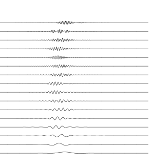
Figure 1: Localized contributions to beam motion.

2 Quasiclassical Evolution

Let us consider classical and quantum dynamics in phase space $\Omega=R^{2m}$ with coordinates $(x,\xi)$ and generated by Hamiltonian ${\cal H}(x,\xi)\in C^{\infty}(\Omega;R)$. If $\Phi^{\cal H}_{t}:\Omega\longrightarrow\Omega$ is (classical) flow then time evolution of any bounded classical observable or symbol $b(x,\xi)\in C^{\infty}(\Omega,R)$ is given by $b_{t}(x,\xi)=b(\Phi^{\cal H}_{t}(x,\xi))$. Let $H=Op^{W}({\cal H})$ and $B=Op^{W}(b)$ are the self-adjoint operators or quantum observables in $L^{2}(R^{n})$, representing the Weyl quantization of the symbols ${\cal H},b$ [12]

$$(Bu)(x)=\frac{1}{(2\pi\hbar)^{n}}\int_{R^{2n}}b\left(\frac{x+y}{2},\xi\right)\cdot$$

$$e^{i<(x-y),\xi>/\hbar}u(y)\mathrm{d}y\mathrm{d}\xi,$$

where $u\in S(R^{n})$ and $B_{t}=e^{iHt/\hbar}Be^{-iHt/\hbar}$ be the Heisenberg observable or quantum evolution of the observable $B$ under unitary group generated by $H$. $B_{t}$ solves the Heisenberg equation of motion $\dot{B}_{t}=({i}/{\hbar})[H,B_{t}].$ Let $b_{t}(x,\xi;\hbar)$ is a symbol of $B_{t}$ then we have the following equation for it

$$\dot{b}_{t}=\{{\cal H},b_{t}\}_{M},$$ (1)

with the initial condition $b_{0}(x,\xi,\hbar)=b(x,\xi)$. Here $\{f,g\}_{M}(x,\xi)$ is the Moyal brackets of the observables $f,g\in C^{\infty}(R^{2n})$, $\{f,g\}_{M}(x,\xi)=f\sharp g-g\sharp f$, where $f\sharp g$ is the symbol of the operator product and is presented by the composition of the symbols $f,g$

$$(f\sharp g)(x,\xi)=\frac{1}{(2\pi\hbar)^{n/2}}\int_{R^{4n}}e^{-i<r,\rho>/\hbar+i<\omega,\tau>/\hbar}$$

$$\cdot f(x+\omega,\rho+\xi)\cdot g(x+r,\tau+\xi)\mathrm{d}\rho\mathrm{d}\tau\mathrm{d}r\mathrm{d}\omega.$$

For our problems it is useful that $\{f,g\}_{M}$ admits the formal expansion in powers of $\hbar$:

$$\{f,g\}_{M}(x,\xi)\sim\{f,g\}+2^{-j}\cdot$$

$$\sum_{|\alpha+\beta|=j\geq 1}(-1)^{|\beta|}\cdot(\partial^{\alpha}_{\xi}fD^{\beta}_{x}g)\cdot(\partial^{\beta}_{\xi}gD^{\alpha}_{x}f),$$

where $\alpha=(\alpha_{1},\dots,\alpha_{n})$ is a multi-index, $|\alpha|=\alpha_{1}+\dots+\alpha_{n}$, $D_{x}=-i\hbar\partial_{x}$. So, evolution (1) for symbol $b_{t}(x,\xi;\hbar)$ is

$$\dot{b}_{t}=\{{\cal H},b_{t}\}+\frac{1}{2^{j}}\sum_{|\alpha|+\beta|=j\geq 1}(-1)^{|\beta|}\cdot$$ (2)

$$\hbar^{j}(\partial^{\alpha}_{\xi}{\cal H}D_{x}^{\beta}b_{t})\cdot(\partial^{\beta}_{\xi}b_{t}D_{x}^{\alpha}{\cal H}).$$

At $\hbar=0$ this equation transforms to classical Liouville equation

$$\dot{b}_{t}=\{{\cal H},b_{t}\}.$$ (3)

Equation (2) plays a key role in many quantum (semiclassical) problem. Our approach to solution of systems (2), (3) is based on our technique from [11] and very useful linear parametrization for differential operators which we present now. Let us consider multiresolution representation $\dots\subset V_{2}\subset V_{1}\subset V_{0}\subset V_{-1}\subset V_{-2}\dots$. Let T be an operator $T:L^{2}(R)\rightarrow L^{2}(R)$, with the kernel $K(x,y)$ and $P_{j}:L^{2}(R)\rightarrow V_{j}$ $(j\in Z)$ is projection operators on the subspace $V_{j}$ corresponding to j level of resolution: $(P_{j}f)(x)=\sum_{k}<f,\varphi_{j,k}>\varphi_{j,k}(x).$ Let $Q_{j}=P_{j-1}-P_{j}$ is the projection operator on the subspace $W_{j}$ then we have the following ”microscopic or telescopic” representation of operator T which takes into account contributions from each level of resolution from different scales starting with coarsest and ending to finest scales [13]: $T=\sum_{j\in Z}(Q_{j}TQ_{j}+Q_{j}TP_{j}+P_{j}TQ_{j}).$ We remember that this is a result of presence of affine group inside this construction. The non-standard form of operator representation [13] is a representation of an operator T as a chain of triples $T=\{A_{j},B_{j},\Gamma_{j}\}_{j\in Z}$, acting on the subspaces $V_{j}$ and $W_{j}$: $A_{j}:W_{j}\rightarrow W_{j},B_{j}:V_{j}\rightarrow W_{j},\Gamma_{j}:W_{j}\rightarrow V_{j},$ where operators $\{A_{j},B_{j},\Gamma_{j}\}_{j\in Z}$ are defined as $A_{j}=Q_{j}TQ_{j},\quad B_{j}=Q_{j}TP_{j},\quad\Gamma_{j}=P_{j}TQ_{j}.$ The operator $T$ admits a recursive definition via

$$T_{j}=\left(\begin{array}[]{cc}A_{j+1}&B_{j+1}\\ \Gamma_{j+1}&T_{j+1}\end{array}\right),$$

where $T_{j}=P_{j}TP_{j}$ and $T_{j}$ works on $V_{j}:V_{j}\rightarrow V_{j}$. It should be noted that operator $A_{j}$ describes interaction on the scale $j$ independently from other scales, operators $B_{j},\Gamma_{j}$ describe interaction between the scale j and all coarser scales, the operator $T_{j}$ is an ”averaged” version of $T_{j-1}$. We may compute such non-standard representations of operator $\mathrm{d}/\mathrm{d}x$ in the wavelet bases by solving only the system of linear algebraical equations. Let $r_{\ell}=\int\varphi(x-\ell)\frac{\mathrm{d}}{\mathrm{d}x}\varphi(x)\mathrm{d}x,\ell\in Z.$ Then, the representation of $d/dx$ is completely determined by the coefficients $r_{\ell}$ or by representation of $d/dx$ only on the subspace $V_{0}$. The coefficients $r_{\ell},\ell\in Z$ satisfy the usual system of linear algebraical equations. For the representation of operator $d^{n}/dx^{n}$ we have the similar reduced linear system of equations. Then finally we have for action of operator $T_{j}(T_{j}:V_{j}\rightarrow V_{j})$ on sufficiently smooth function $f$:

$$(T_{j}f)(x)=\sum_{k\in Z}\left(2^{-j}\sum_{\ell}r_{\ell}f_{j,k-\ell}\right)\varphi_{j,k}(x),$$

where $\varphi_{j,k}(x)=2^{-j/2}\varphi(2^{-j}x-k)$ is wavelet basis and

$$f_{j,k-1}=2^{-j/2}\int f(x)\varphi(2^{-j}x-k+\ell)\mathrm{d}x$$

are wavelet coefficients. So, we have simple linear parametrization of matrix representation of our differential operator in wavelet basis and of the action of this operator on arbitrary vector in our functional space. Then we may use such representation in all quasiclassical calculations.

3 Wigner Transform

According to Weyl transform (observable-symbol) state or wave function corresponds to Wigner function, which is analog of classical phase-space distribution. If $\psi(x,t),x\in R^{n}$ satisfies the Schroedinger equation

$$i\hbar\partial_{t}\psi=-(\hbar^{2}/2)\triangle\psi+V\psi$$ (4)

and W is the Wigner transform of $\psi$

$$W(t,x,\nu)= \int e^{-i\nu y}\bar{\psi}(t,x+(\hbar/2)y)\cdot$$ (5)

$$\psi(t,x-(\hbar/2)y)\mathrm{d}y,$$

then W satisfies the pseudo-differential ($\psi$DO) Wigner equation

$$\partial_{t}W+\upsilon\partial_{x}W-(i/\hbar)P(V)W=0,$$ (6)

where $\psi$DO operator $P(V)$ is

$$P(V)f(x,\nu)=\frac{1}{(2\pi)^{n}}\int e^{-i\nu y}\Big{[}V(x+\frac{\hbar}{2}y)-$$

$$V(x-\frac{\hbar}{2}y)\Big{]}\cdot\Big{(}\int e^{iy\xi}f(x,\xi)\mathrm{d}\xi\Big{)}\mathrm{d}y$$ (7)

In quasiclassical limit $\hbar\to 0$ the operator $P(V)$ converges to $-\partial_{x}V\cdot\partial_{\nu}$. We consider it in [11]. On Fig. 2 we present calculations [14] of Wigner transform for beam motion, represented by four gaussians, which explicitly demonstrates quantum inteference in the phase space.

We give more details in [11].

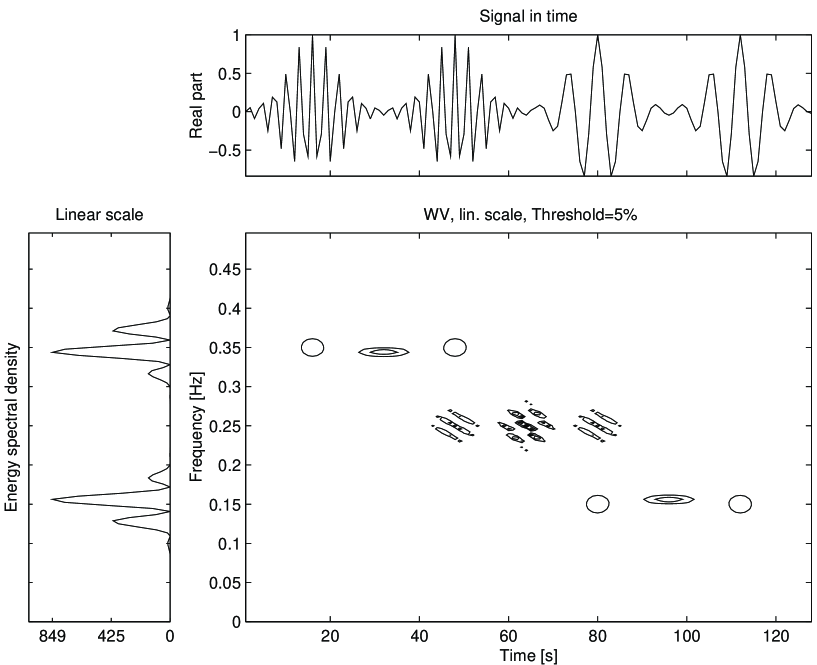
Figure 2: Wigner transform

We would like to thank Professor James B. Rosenzweig and Mrs. Melinda Laraneta for nice hospitality, help and support during UCLA ICFA Workshop.

References

- [1] C. Hill, Los Alamos preprint: hep-ph/0002230, S. Khan, M. Pusterla, physics/9910026.
- [2] A.N. Fedorova and M.G. Zeitlin, ’Wavelets in Optimization and Approximations’, Math. and Comp. in Simulation, 46, 527, 1998.
- [3] A.N. Fedorova and M.G. Zeitlin, ’Wavelet Approach to Mechanical Problems. Symplectic Group, Symplectic Topology and Symplectic Scales’, New Applications of Nonlinear and Chaotic Dynamics in Mechanics, 31,101 (Kluwer, 1998).
-
[4]
A.N. Fedorova and M.G. Zeitlin,
’Nonlinear Dynamics of Accelerator via Wavelet
Approach’, CP405, 87 (American Institute of Physics, 1997).
Los Alamos preprint, physics/9710035. - [5] A.N. Fedorova, M.G. Zeitlin and Z. Parsa, ’Wavelet Approach to Accelerator Problems’, parts 1-3, Proc. PAC97 2, 1502, 1505, 1508 (IEEE, 1998).
- [6] A.N. Fedorova, M.G. Zeitlin and Z. Parsa, Proc. EPAC98, 930, 933 (Institute of Physics, 1998).
-
[7]
A.N. Fedorova, M.G. Zeitlin and Z. Parsa,
Variational Approach in
Wavelet Framework to Polynomial
Approximations of Nonlinear Accelerator Problems.
CP468, 48 ( American Institute of Physics, 1999).
Los Alamos preprint, physics/990262 -
[8]
A.N. Fedorova, M.G. Zeitlin and Z. Parsa,
Symmetry, Hamiltonian
Problems and Wavelets in
Accelerator Physics.
CP468, 69 (American Institute of Physics, 1999).
Los Alamos preprint, physics/990263 -
[9]
A.N. Fedorova and M.G. Zeitlin,
Nonlinear Accelerator Problems
via Wavelets, parts 1-8,
Proc. PAC99,
1614, 1617, 1620, 2900, 2903,
2906, 2909, 2912 (IEEE/APS, New York, 1999).
Los Alamos preprints: physics/9904039, physics/9904040, physics/9904041, physics/9904042, physics/9904043, physics/9904045, physics/9904046, physics/9904047. - [10] A.N. Fedorova and M.G. Zeitlin, Los Alamos preprint: physics/0003095.
- [11] A.N. Fedorova, M.G. Zeitlin, in press
- [12] D. Sternheimer, Los Alamos preprint: math/9809056.
- [13] G. Beylkin, R.Coifman, V. Rokhlin, Comm. Pure Appl. Math.,44, 141, 1991
- [14] F. Auger, e.a., Time-frequency Toolbox, CNRS/Rice Univ., 1996