1 Problem

Consider a variant on the physical situation of “slow light” [1, 2] in which two closely spaced spectral lines are now both optically pumped to show that the group velocity can be negative at the central frequency, which leads to apparent superluminal behavior.

1.1 Negative Group Velocity

In more detail, consider a classical model of matter in which spectral lines are associated with oscillators. In particular, consider a gas with two closely spaced spectral lines of angular frequencies $\omega_{1,2}=\omega_{0}\pm\Delta/2$, where $\Delta\ll\omega_{0}$. Each line has the same damping constant (and spectral width) $\gamma$.

Ordinarily, the gas would exhibit strong absorption of light in the vicinity of the spectral lines. But suppose that lasers of frequencies $\omega_{1}$ and $\omega_{2}$ pump the both oscillators into inverted populations. This can be described classically by assigning negative oscillator strengths to these oscillators [3].

Deduce an expression for the group velocity $v_{g}(\omega_{0})$ of a pulse of light centered on frequency $\omega_{0}$ in terms of the (univalent) plasma frequency $\omega_{p}$ of the medium, given by

$$\omega_{p}^{2}={4\pi Ne^{2}\over m},$$ (1)

where $N$ is the number density of atoms, and $e$ and $m$ are the charge and mass of an electron. Give a condition on the line separation $\Delta$ compared to the line width $\gamma$ such that the group velocity $v_{g}(\omega_{0})$ is negative.

In a recent experiment by Wang et al. [4], a group velocity of $v_{g}=-c/310$, where $c$ is the speed of light in vacuum, was demonstrated in cesium vapor using a pair of spectral lines with separation $\Delta/2\pi\approx 2$ MHz and linewidth $\gamma/2\pi\approx 0.8$ MHz.

1.2 Propagation of a Monochromatic Plane Wave

Consider a wave with electric field $E_{0}e^{i\omega(z/c-t)}$ that is incident from $z<0$ on a medium that extends from $z=0$ to $a$. Ignore reflection at the boundaries, as is reasonable if the index of refraction $n(\omega)$ is near unity. Particularly simple results can be obtained when you make the (unphysical) assumption that the $\omega n(\omega)$ varies linearly with frequency about a central frequency $\omega_{0}$. Deduce a transformation that has a frequency-dependent part and a frequency-independent part between the phase of the wave for $z<0$ to that of the wave inside the medium, and to that of the wave in the region $a<z$.

1.3 Fourier Analysis

Apply the transformations between an incident monochromatic wave and the wave in and beyond the medium to the Fourier analysis of an incident pulse of form $f(z/c-t)$.

1.4 Propagation of a Sharp Wave Front

In the approximation that $\omega n$ varies linearly with $\omega$, deduce the waveforms in the regions $0<z<a$ and $a<z$ for an incident pulse $\delta(z/c-t)$, where $\delta$ is the Dirac delta function. Show that the pulse emerges out of the gain region at $z=a$ at time $t=a/v_{g}$, which appears to be earlier than when it enters this region if the group velocity is negative. Show also that inside the negative group velocity medium a pulse propagates backwards from $z=a$ at time $t=a/v_{g}<0$ to $z=0$ at $t=0$, at which time it appears to annihilate the incident pulse.

1.5 Propagation of a Gaussian Pulse

As a more physical example, deduce the waveforms in the regions $0<z<a$ and $a<z$ for a Gaussian incident pulse $E_{0}e^{-(z/c-t)^{2}/2\tau^{2}}e^{i\omega_{0}(z/c-t)}$. Carry the frequency expansion of $\omega n(\omega)$ to second order to obtain conditions of validity of the analysis such as maximum pulsewidth $\tau$, maximum length $a$ of the gain region, and maximum time of advance of the emerging pulse. Consider the time required to generate a pulse of risetime $\tau$ when assessing whether the time advance in a negative group velocity medium can lead to superluminal signal propagation.

2 Solution

The concept of group velocity appears to have been first enunciated by Hamilton in 1839 in lectures of which only abstracts were published [5]. The first recorded observation of the group velocity of a (water) wave is due to Russell in 1844 [6]. However, widespread awareness of the group velocity dates from 1876 when Stokes used its as the topic of a Smith’s Prize examination paper [7]. The early history of group velocity has been reviewed by Havelock [8].

H. Lamb [9] credits A. Schuster with noting in 1904 that a negative group velocity, i.e., a group velocity of opposite sign to that of the phase velocity, is possible due to anomalous dispersion. Von Laue [10] made a similar comment in 1905. Lamb gave two examples of strings subject to external potentials that exhibit negative group velocities. These early considerations assumed that in case of a wave with positive group and phase velocities incident on the anomalous medium, energy would be transported into the medium with a positive group velocity, and so there would be waves with negative phase velocity inside the medium. Such negative phase velocity waves are formally consistent with Snell’s law [11] (since $\theta_{t}=\sin^{-1}[(n_{i}/n_{t})\sin\theta_{i}]$ can be in either the first or second quadrant), but they seemed physically implausible and the topic was largely dropped.

Present interest in negative group velocity a based on anomalous dispersion in a gain medium, where the sign of the phase velocity is the same for incident and transmitted waves, and energy flows inside the gain medium in the opposite direction to the incident energy flow in vacuum.

The propagation of electromagnetic waves at frequencies near those of spectral lines of a medium was first extensively discussed by Sommerfeld and Brillouin [12], with emphasis on the distinction between signal velocity and group velocity when the latter exceeds $c$. The solution presented here is based on the work of Garrett and McCumber [13], as extended by Chiao et al.  [14, 15]. A discussion of negative group velocity in electronic circuits has been given by Mitchell and Chiao [16].

2.1 Negative Group Velocity

In a medium of index of refraction $n(\omega)$, the dispersion relation can be written

$$k={\omega n\over c},$$ (2)

where $k$ is the wave number. The group velocity is then given by

$$v_{g}=Re\left[{d\omega\over dk}\right]={1\over Re[dk/d\omega]}={c\over Re[d(\omega n)/d\omega]}={c\over n+\omega Re[dn/d\omega]}.$$ (3)

We see from eq. (3) that if the index of refraction decreases rapidly enough with frequency, the group velocity can be negative. It is well known that the index of refraction decreases rapidly with frequency near an absorption line, where “anomalous” wave propagation effects can occur [12]. However, the absorption makes it difficult to study these effects. The insight of Garrett and McCumber [13] and of Chiao et al. [14, 15, 17, 18, 19] is that demonstrations of negative group velocity are possible in media with inverted populations, so that gain rather than absorption occurs at the frequencies of interest. This was dramatically realized in the experiment of Wang et al. [4] by use of a closely spaced pair of gain lines, as perhaps first suggested by Steinberg and Chiao [17].

We use a classical oscillator model for the index of refraction. The index $n$ is the square root of the dielectric constant $\epsilon$, which is in turn related to the atomic polarizability $\alpha$ according to

$$D=\epsilon E=E+4\pi P=E(1+4\pi N\alpha),$$ (4)

(in Gaussian units) where $D$ is the electric displacement, $E$ is the electric field and $P$ is the polarization density. Then, the index of refraction of a dilute gas is

$$n=\sqrt{\epsilon}\approx 1+2\pi N\alpha.$$ (5)

The polarizability $\alpha$ is obtained from the electric dipole moment $p=ex=\alpha E$ induced by electric field $E$. In the case of a single spectral line of frequency $\omega_{j}$, we say that an electron is bound to the (fixed) nucleus by a spring of constant $K=m\omega_{j}^{2}$, and that the motion is subject to the damping force $-m\gamma_{j}\dot{x}$, where the dot indicates differentiation with respect to time. The equation of motion in the presence of an electromagnetic wave of frequency $\omega$ is

$$\ddot{x}+\gamma_{j}\dot{x}+\omega_{j}^{2}x={eE\over m}={eE_{0}\over m}e^{i\omega t}.$$ (6)

Hence,

$$x={eE\over m}{1\over\omega_{j}^{2}-\omega^{2}-i\gamma_{j}\omega}={eE\over m}{\omega_{j}^{2}-\omega^{2}+i\gamma_{j}\omega\over(\omega_{j}^{2}-\omega^{2})^{2}+\gamma_{j}^{2}\omega^{2}},$$ (7)

and the polarizability is

$$\alpha={e^{2}\over m}{\omega_{j}^{2}-\omega^{2}+i\gamma_{j}\omega\over(\omega_{j}^{2}-\omega^{2})^{2}+\gamma_{j}^{2}\omega^{2}}.$$ (8)

In the present problem, we have two spectral lines, $\omega_{1,2}=\omega_{0}\pm\Delta/2$, both of oscillator strength $-1$ to indicate that the populations of both lines are inverted, with damping constants $\gamma_{1}=\gamma_{2}=\gamma$. In this case, the polarizability is given by

$$\alpha = -{e^{2}\over m}{(\omega_{0}-\Delta/2)^{2}-\omega^{2}+i\gamma\omega\over((\omega_{0}-\Delta/2)^{2}-\omega^{2})^{2}+\gamma^{2}\omega^{2}}-{e^{2}\over m}{(\omega_{0}+\Delta/2)^{2}-\omega^{2}+i\gamma\omega\over((\omega_{0}+\Delta/2)^{2}-\omega^{2})^{2}+\gamma^{2}\omega^{2}}$$ (9)

$$\approx -{e^{2}\over m}{\omega_{0}^{2}-\Delta\omega_{0}-\omega^{2}+i\gamma\omega\over(\omega_{0}^{2}-\Delta\omega_{0}-\omega^{2})^{2}+\gamma^{2}\omega^{2}}-{e^{2}\over m}{\omega_{0}^{2}+2\Delta\omega_{0}-\omega^{2}+i\gamma\omega\over(\omega_{0}^{2}+\Delta\omega_{0}-\omega^{2})^{2}+\gamma^{2}\omega^{2}},$$

where the approximation is obtained by the neglect of terms in $\Delta^{2}$ compared to those in $\Delta\omega_{0}$.

For a probe beam at frequency $\omega$, the index of refraction (5) has the form

$$n(\omega)\approx 1-{\omega_{p}^{2}\over 2}\left[{\omega_{0}^{2}-\Delta\omega_{0}-\omega^{2}+i\gamma\omega\over(\omega_{0}^{2}-\Delta\omega_{0}-\omega^{2})^{2}+\gamma^{2}\omega^{2}}+{\omega_{0}^{2}+\Delta\omega_{0}-\omega^{2}+i\gamma\omega\over(\omega_{0}^{2}+\Delta\omega_{0}-\omega^{2})^{2}+\gamma^{2}\omega^{2}}\right],$$ (10)

where $\omega_{p}$ is the plasma frequency given by eq. (1). This illustrated in Figure 1.

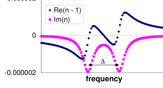
Figure 1: The real and imaginary parts of the index of refraction in a medium with two spectral lines that have been pumped to inverted populations. The lines are separated by angular frequency $\Delta$ and have widths $\gamma=0.4\Delta$.

The index at the central frequency $\omega_{0}$ is

$$n(\omega_{0})\approx 1-i{\omega_{p}^{2}\gamma\over(\Delta^{2}+\gamma^{2})\omega_{0}}\approx 1-i{\omega_{p}^{2}\over\Delta^{2}}{\gamma\over\omega_{0}},$$ (11)

where the second approximation holds when $\gamma\ll\Delta$. The electric field of a continuous probe wave then propagates according to

$$E(z,t)=e^{i(kz-\omega_{0}t)}=e^{i\omega_{0}(n(\omega_{0})z/c-t)}\approx e^{z/[\Delta^{2}c/\gamma\omega_{p}^{2}]}e^{i\omega_{0}(z/c-t)}.$$ (12)

From this we see that at frequency $\omega_{0}$ the phase velocity is $c$, and the medium has an amplitude gain length $\Delta^{2}c/\gamma\omega_{p}^{2}$.

To obtain the group velocity (3) at frequency $\omega_{0}$, we need the derivative

$${d(\omega n)\over d\omega}\biggr{|}_{\omega_{0}}\approx 1-{2\omega_{p}^{2}(\Delta^{2}-\gamma^{2})\over(\Delta^{2}+\gamma^{2})^{2}},$$ (13)

where we have neglected terms in $\Delta$ and $\gamma$ compared to $\omega_{0}$. From eq. (3), we see that the group velocity can be negative if

$${\Delta^{2}\over\omega_{p}^{2}}-{\gamma^{2}\over\omega_{p}^{2}}\geq{1\over 2}\left({\Delta^{2}\over\omega_{p}^{2}}+{\gamma^{2}\over\omega_{p}^{2}}\right)^{2}.$$ (14)

The boundary of the allowed region (14) in $(\Delta^{2},\gamma^{2})$ space is a parabola whose axis is along the line $\gamma^{2}=-\Delta^{2}$, as shown in Fig. 2. For the physical region $\gamma^{2}\geq 0$, the boundary is given by

$${\gamma^{2}\over\omega_{p}^{2}}=\sqrt{1+4{\Delta^{2}\over\omega_{p}^{2}}}-1-{\Delta^{2}\over\omega_{p}^{2}}.$$ (15)

Thus, to have a negative group velocity, we must have

$$\Delta\leq\sqrt{2}\omega_{p},$$ (16)

which limit is achieved when $\gamma=0$; the maximum value of $\gamma$ is $0.5\omega_{p}$ when $\Delta=0.866\omega_{p}$.

Figure 2: The allowed region (14) in $(\Delta^{2},\gamma^{2})$ space such that the group velocity is negative.

Near the boundary of the negative group velocity region, $\left|v_{g}\right|$ exceeds $c$, which alerts us to concerns of superluminal behavior. However, as will be seen in the following sections, the effect of a negative group velocity is more dramatic when $\left|v_{g}\right|$ is small rather than large.

The region of recent experimental interest is $\gamma\ll\Delta\ll\omega_{p}$, for which eqs. (3) and (13) predict that

$$v_{g}\approx-{c\over 2}{\Delta^{2}\over\omega_{p}^{2}}.$$ (17)

A value of $v_{g}\approx-c/310$ as in the experiment of Wang corresponds to $\Delta/\omega_{p}\approx 1/12$. In this case, the gain length $\Delta^{2}c/\gamma\omega_{p}^{2}$ was approximately 40 cm.

For later use we record the second derivative,

$${d^{2}(\omega n)\over d\omega^{2}}\biggr{|}_{\omega_{0}}\approx 8i{\omega_{p}^{2}\gamma(3\Delta^{2}-\gamma^{2})\over(\Delta^{2}+\gamma^{2})^{3}}\approx 24i{\omega_{p}^{2}\over\Delta^{2}}{\gamma\over\Delta^{2}}$$ (18)

where the second approximation holds if $\gamma\ll\Delta$.

2.2 Propagation of a Monochromatic Plane Wave

To illustrate the optical properties of a medium with negative group velocity, we consider the propagation of an electromagnetic wave through it. The medium extends from $z=0$ to $a$, and is surrounded by vacuum. Because the index of refraction (10) is near unity in the frequency range of interest, we ignore reflections at the boundaries of the medium.

A monochromatic plane wave of frequency $\omega$ and incident from $z<0$ propagates with phase velocity $c$ in vacuum. Its electric field can be written

$$E_{\omega}(z,t)=E_{0}e^{i\omega z/c}e^{-i\omega t}\qquad(z<0).$$ (19)

Inside the medium this wave propagates with phase velocity $c/n(\omega)$ according to

$$E_{\omega}(z,t)=E_{0}e^{i\omega nz/c}e^{-i\omega t}\qquad(0<z<a),$$ (20)

where the amplitude is unchanged since we neglect the small reflection at the boundary $z=0$. When the wave emerges into vacuum at $z=a$, the phase velocity is again $c$, but it has accumulated a phase lag of $(\omega/c)(n-1)a$, and so appears as

$$E_{\omega}(z,t)=E_{0}e^{i\omega a(n-1)/c}e^{i\omega z/c}e^{-i\omega t}=E_{0}e^{i\omega an/c}e^{-i\omega(t-(z-a)/c)}\qquad(a<z).$$ (21)

It is noteworthy that a monochromatic wave for $z>a$ has the same form as that inside the medium if we make the frequency-independent substitutions

$$z\to a,\qquad\mbox{and}\qquad t\to t-{z-a\over c}.$$ (22)

Since an arbitrary waveform can be expressed in terms of monochromatic plane waves via Fourier analysis, we can use these substitutions to convert any wave in the region $0<z<a$ to its continuation in the region $a<z$.

A general relation can be deduced in the case where the second and higher derivatives of $\omega n(\omega)$ are very small. We can then write

$$\omega n(\omega)\approx\omega_{0}n(\omega_{0})+{c\over v_{g}}(\omega-\omega_{0}),$$ (23)

where $v_{g}$ is the group velocity for a pulse with central frequency $\omega_{0}$. Using this in eq. (20), we have

$$E_{\omega}(z,t)\approx E_{0}e^{i\omega_{0}z(n(\omega_{0})/c-1/v_{g})}e^{i\omega z/v_{g}}e^{-i\omega t}\qquad(0<z<a).$$ (24)

In this approximation, the Fourier component $E_{\omega}(z)$ at frequency $\omega$ of a wave inside the gain medium is related to that of the incident wave by replacing the frequency dependence $e^{i\omega z/c}$ by $e^{i\omega z/v_{g}}$, i.e., by replacing $z/c$ by $z/v_{g}$, and multiplying by the frequency-independent phase factor $e^{i\omega_{0}z(n(\omega_{0})/c-1/v_{g})}$. Then, using transformation (22), the wave that emerges into vacuum beyond the medium is

$$E_{\omega}(z,t)\approx E_{0}e^{i\omega_{0}a(n(\omega_{0})/c-1/v_{g})}e^{i\omega(z/c-a(1/c-1/v_{g}))}e^{-i\omega t}\qquad(a<z).$$ (25)

The wave beyond the medium is related to the incident wave by multiplying by a frequency-independent phase, and by replacing $z/c$ by $z/c-a(1/c-1/v_{g})$ in the frequency-dependent part of the phase.

The effect of the medium on the wave as described by eqs. (24)-(25) has been called “rephasing” [4].

2.3 Fourier Analysis and “Rephasing”

The transformations between the monochromatic incident wave (19) and its continuation in and beyond the medium, (24) and (25), imply that an incident wave

$$E(z,t)=f(z/c-t)=\int_{-\infty}^{\infty}d\omega\,E_{\omega}(z)e^{-i\omega t}\qquad(z<0),$$ (26)

whose Fourier components are given by

$$E_{\omega}(z)={1\over 2\pi}\int_{-\infty}^{\infty}dE(z,t)e^{i\omega t}dt,$$ (27)

propagates as

$$E(z,t)\approx\left\{\begin{array}[]{ll}f(z/c-t)&\qquad(z<0),\\ e^{i\omega_{0}z(n(\omega_{0})/c-1/v_{g})}f(z/v_{g}-t)&\qquad(0<z<a),\\ e^{i\omega_{0}a(n(\omega_{0})/c-1/v_{g})}f(z/c-t-a(1/c-1/v_{g}))&\qquad(a<z).\end{array}\right.$$ (31)

An interpretation of eq. (31) in terms of “rephasing” is as follows. Fourier analysis tells us that the maximum amplitude of a pulse made of waves of many frequencies, each of the form $E_{\omega}(z,t)=E_{0}(\omega)e^{i\phi(\omega)}=E_{0}(\omega)e^{i(k(\omega)z-\omega t+\phi_{0}(\omega))}$ with $E_{0}\geq 0$, is determined by adding the amplitudes $E_{0}(\omega)$. This maximum is achieved only if there exists points $(z,t)$ such that all phases $\phi(\omega)$ have the same value.

For example, we consider a pulse in the region $z<0$ whose maximum occurs when the phases of all component frequencies vanish, as shown at the left of Fig. 3. Referring to eq. (19), we see that the peak occurs when $z=ct$. As usual, we say that the group velocity of this wave is $c$ in vacuum.

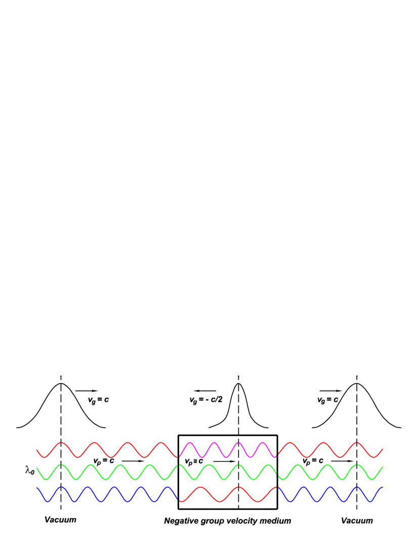
Figure 3: A snapshot of three Fourier components of a pulse in the vicinity of a negative group velocity medium. The component at the central wavelength $\lambda_{0}$ is unaltered by the medium, but the wavelength of a longer wavelength component is shortened, and that of a shorter wavelength component is lengthened. Then, even when the incident pulse has not yet reached the medium, there can be a point inside the medium at which all components have the same phase, and a peak appears. Simultaneously, there can be a point in the vacuum region beyond the medium at which the Fourier components are again all in phase, and a third peak appears. The peaks in the vacuum regions move with group velocity $v_{g}=c$, but the peak inside the medium moves with a negative group velocity, shown as $v_{g}=-c/2$ in the figure. The phase velocity $v_{p}$ is $c$ in vacuum, and close to $c$ in the medium.

Inside the medium, eq. (24) describes the phases of the components, which all have a common frequency-independent phase $\omega_{0}z(n(\omega_{0})/c-1/v_{g})$ at a given $z$, as well as a frequency-dependent part $\omega(z/v_{g}-t)$. The peak of the pulse occurs when all the frequency-dependent phases vanish; the overall frequency-independent phase does not affect the pulse size. Thus, the peak of the pulse propagates within the medium according to $z=v_{g}t$. The velocity of the peak is $v_{g}$, the group velocity of the medium, which can be negative.

The “rephasing” (24) within the medium changes the wavelengths of the component waves. Typically the wavelength increases, and by greater amounts at longer wavelengths. A longer time is required before the phases of the waves all becomes the same at some point $z$ inside the medium, so in a normal medium the velocity of the peak appears to be slowed down. But in a negative group velocity medium, wavelengths short compared to $\lambda_{0}$ are lengthened, long waves are shortened, and the velocity of the peak appears to be reversed.

By a similar argument, eq. (25) tells us that in the vacuum region beyond the medium the peak of the pulse propagates according to $z=ct+a(1/c-1/v_{g})$. The group velocity is again $c$, but the “rephasing” within the medium results in a shift of the position of the peak by amount $a(1/c-1/v_{g})$. In a normal medium where $0<v_{g}\leq c$ the shift is negative; the pulse appears to have been delayed during its passage through the medium. But after a negative group velocity medium, the pulse appears to have advanced!

This advance is possible because in the Fourier view, each component wave extends over all space, even if the pulse appears to be restricted. The unusual “rephasing” in a negative group velocity medium shifts the phases of the frequency components of the wave train in the region ahead of the nominal peak such that the phases all coincide, and a peak is observed, at times earlier than expected at points beyond the medium.

As shown in Fig. 3 and further illustrated in the examples below, the “rephasing” can result in the simultaneous appearance of peaks in all three regions.

2.4 Propagation of a Sharp Wave Front

To assess the effect of a medium with negative group velocity on the propagation of a signal, we first consider a waveform with a sharp front, as recommended by Sommerfeld and Brillouin [12].

As an extreme but convenient example, we take the incident pulse to be a Dirac delta function, $E(z,t)=E_{0}\delta(z/c-t)$. Inserting this in eq. (31), which is based on the linear approximation (23), we find

$$E(z,t)\approx\left\{\begin{array}[]{ll}E_{0}\delta(z/c-t)&\qquad(z<0),\\ E_{0}e^{i\omega_{0}z(n(\omega_{0})/c-1/v_{g})}\delta(z/v_{g}-t)&\qquad(0<z<a),\\ E_{0}e^{i\omega_{0}a(n(\omega_{0})/c-1/v_{g})}\delta(z/c-t-a(1/c-1/v_{g}))&\qquad(a<z),\end{array}\right.$$ (35)

According to eq. (35), the delta-function pulse emerges from the medium at $z=a$ at time $t=a/v_{g}$. If the group velocity is negative, the pulse emerges from the medium before it enters at $t=0$!

A sample history of (Gaussian) pulse propagation is illustrated in Fig. 4. Inside the negative group velocity medium, an (anti)pulse propagates backwards in space from $z=a$ at time $t=a/v_{g}<0$ to $z=0$ at time $t=0$, at which point it appears to annihilate the incident pulse.

This behavior is analogous to barrier penetration by a relativistic electron [20] in which an electron can emerge from the far side of the barrier earlier than it hits the near side, if the electron emission at the far side is accompanied by positron emission, and the positron propagates within the barrier so as to annihilate the incident electron at the near side. In the Wheeler-Feynman view, this process involves only a single electron which propagates backwards in time when inside the barrier. In this spirit, we might say that pulses propagate backwards in time (but forward in space) inside a negative group velocity medium.

The Fourier components of the delta function are independent of frequency, so the advanced appearance of the sharp wavefront as described by eq. (35) can occur only for a gain medium such that the index of refraction varies linearly at all frequencies. If such a medium existed with negative slope $dn/d\omega$, then eq. (35) would constitute superluminal signal propagation.

However, from Fig. 1 we see that a linear approximation to the index of refraction is reasonable in the negative group velocity medium only for $\left|\omega-\omega_{0}\right|\mathrel{\vbox{\kern 0.0pt\hbox{$<$} \kern 0.0pt\hbox{$\sim$} }}\Delta/2$. The sharpest wavefront that can be supported within this bandwidth has characteristic risetime $\tau\approx 1/\Delta$.

For the experiment of Wang et al. where $\Delta/2\pi\approx 10^{6}$ Hz, an analysis based on eq. (23) would be valid only for pulses with $\tau\mathrel{\vbox{\kern 0.0pt\hbox{$>$} \kern 0.0pt\hbox{$\sim$} }}0.1\ \mu$s. Wang et al. used a pulse with $\tau\approx 1\ \mu$s, close to the minimum value for which eq. (23) is a reasonable approximation.

Since a negative group velocity can only be experienced over a limited bandwidth, very sharp wavefronts must be excluded from discussion of signal propagation. However, it is well known [12] that great care must be taken when discussing the signal velocity if the waveform is not sharp.

2.5 Propagation of a Gaussian Pulse

We now consider a Gaussian pulse of temporal length $\tau$ centered on frequency $\omega_{0}$ (the carrier frequency), for which the incident waveform is

$$E(z,t)=E_{0}e^{-(z/c-t)^{2}/2\tau^{2}}e^{i\omega_{0}z/c}e^{-i\omega_{0}t}\qquad(z<0),$$ (36)

Inserting this in eq. (31) we find

$$E(z,t)=\left\{\begin{array}[]{ll}E_{0}e^{-(z/c-t)^{2}/2\tau^{2}}e^{i\omega_{0}(z/c-t)}&\qquad(z<0),\\ E_{0}e^{-(z/v_{g}-t)^{2}/2\tau^{2}}e^{i\omega_{0}(n(\omega_{0})z/c-t)}&\qquad(0<z<a),\\ E_{0}e^{i\omega_{0}a(n(\omega_{0})-1)/c}e^{-(z/c-a(1/c-1/v_{g})-t)^{2}/2\tau^{2}}e^{i\omega_{0}(z/c-t)}&\qquad(a<z).\end{array}\right.$$ (40)

The factor $e^{i\omega_{0}a(n(\omega_{0})-1)/c}$ in eq. (40) for $a<z$ becomes $e^{\omega_{p}^{2}\gamma a/\Delta^{2}c}$ using eq. (11), and represents a small gain due to traversing the negative group velocity medium. In the experiment of Wang et al. this factor was only 1.16.

We have already noted in the previous section that the linear approximation to $\omega n(\omega)$ is only good over a frequency interval about $\omega_{0}$ of order $\Delta$, and so eq. (40) for the pulse after the gain medium applies only for pulsewidths

$$\tau\mathrel{\vbox{\kern 0.0pt\hbox{$>$} \kern 0.0pt\hbox{$\sim$} }}{1\over\Delta}.$$ (41)

Further constraints on the validity of eq. (40) can obtained using the expansion of $\omega n(\omega)$ to second order. For this, we repeat the derivation of eq. (40) in slightly more detail. The incident Gaussian pulse (36) has the Fourier decomposition (27)

$$E_{\omega}(z)={\tau\over\sqrt{2\pi}}E_{0}e^{-\tau^{2}(\omega-\omega_{0})^{2}/2}e^{i\omega z/c}\qquad(z<0).$$ (42)

We again extrapolate the Fourier component at frequency $\omega$ into the region $z>0$ using eq. (20), which yields

$$E_{\omega}(z)={\tau\over\sqrt{2\pi}}E_{0}e^{-\tau^{2}(\omega-\omega_{0})^{2}/2}e^{i\omega nz/c}\qquad(0<z<a).$$ (43)

We now approximate the factor $\omega n(\omega)$ by its Taylor expansion through second order:

$$\omega n(\omega)\approx\omega_{0}n(\omega_{0})+{c\over v_{g}}(\omega-\omega_{0})+{1\over 2}{d^{2}(\omega n)\over d\omega^{2}}\Biggr{|}_{\omega_{0}}(\omega-\omega_{0})^{2}.$$ (44)

With this, we find from eqs. (26) and (43) that

$$E(z,t)={E_{0}\over A}e^{-(z/v_{g}-t)^{2}/2A^{2}\tau^{2}}e^{i\omega_{0}n(\omega_{0})z/c}e^{-i\omega_{0}t}\qquad(0<z<a),$$ (45)

where

$$A^{2}(z)=1-i{z\over c\tau^{2}}{d^{2}(\omega n)\over d\omega^{2}}\Biggr{|}_{\omega_{0}}.$$ (46)

The waveform for $z>a$ is obtained from that for $0<z<a$ by the substitutions (22) with the result

$$E(z,t)={E_{0}\over A}e^{i\omega_{0}a(n(\omega_{0})-1)/c}e^{-(z/c-a(1/c-1/v_{g})-t)^{2}/2A^{2}\tau^{2}}e^{i\omega_{0}z/c}e^{-i\omega_{0}t}\qquad(a<z),$$ (47)

where $A$ is evaluated at $z=a$ here. As expected, the forms (45) and (47) revert to those of eq. (40) when $d^{2}(\omega n(\omega_{0}))/d\omega^{2}=0$.

So long as the factor $A(a)$ is not greatly different from unity, the pulse emerges from the medium essentially undistorted, which requires

$${a\over c\tau}\ll{1\over 24}{\Delta^{2}\over\omega_{p}^{2}}{\Delta\over\gamma}\Delta\tau,$$ (48)

using eqs. (18) and (46). In the experiment of Wang et al., this condition is that $a/c\tau\ll 1/120$, which was well satisfied with $a=6$ cm and $c\tau=300$ m.

As in the case of the delta function, the centroid of a Gaussian pulse emerges from a negative group velocity medium at time

$$t={a\over v_{g}}<0,$$ (49)

which is earlier than the time $t=0$ when the centroid enters the medium. In the experiment of Wang et al., the time advance of the pulse was $a/\left|v_{g}\right|\approx 300a/c\approx 6\times 10^{-8}$ s $\approx 0.06\tau$.

If one attempts to observe the negative group velocity pulse inside the medium, the incident wave would be perturbed and the backwards-moving pulse would not be detected. Rather, one must deduce the effect of the negative group velocity medium by observation of the pulse that emerges into the region $z>a$ beyond that medium, where the significance of the time advance (49) is the main issue.

The time advance caused by a negative group velocity medium is larger when $\left|v_{g}\right|$ is smaller. It is possible that $\left|v_{g}\right|>c$, but this gives a smaller time advance than when the negative group velocity is such that $\left|v_{g}\right|<c$. Hence, there is no special concern as to the meaning of negative group velocity when $\left|v_{g}\right|>c$.

The maximum possible time advance $t_{\rm max}$ by this technique can be estimated from eqs. (17), (48) and (49) as

$${t_{\rm max}\over\tau}\approx{1\over 12}{\Delta\over\gamma}\Delta\tau\approx 1.$$ (50)

The pulse can advance by at most a few risetimes due to passage through the negative group velocity medium.

While this aspect of the pulse propagation appears to be superluminal, it does not imply superluminal signal propagation.

In accounting for signal propagation time, the time needed to generate the signal must be included as well. A pulse with a finite frequency bandwidth $\Delta$ takes at least time $\tau\approx 1/\Delta$ to be generated, and so is delayed by a time of order its risetime $\tau$ compared to the case of an idealized sharp wavefront. Thus, the advance of a pulse front in a negative group velocity medium by $\mathrel{\vbox{\kern 0.0pt\hbox{$<$} \kern 0.0pt\hbox{$\sim$} }}\tau$ can at most compensate for the original delay in generating that pulse. The signal velocity, as defined by the path length between the source and detector divided by the overall time from onset of signal generation to signal detection, remains bounded by $c$.

As has been emphasized by Garrett and McCumber [13] and by Chiao [18, 19], the time advance of a pulse emerging from a gain medium is possible because the forward tail of a smooth pulse gives advance warning of the later arrival of the peak. The leading edge of the pulse can be amplified by the gain medium, which gives the appearance of superluminal pulse velocities. However, the medium is merely using information stored in the early part of the pulse during its (lengthy) time of generation to bring the apparent velocity of the pulse closer to $c$.

The effect of the negative group velocity medium can be dramatized in a calculation based on eq. (40) in which the pulse width is narrower than the gain region (in violation of condition (48)), as shown in Fig. 4. Here, the gain region is $0<z<50$, the group velocity is taken to be $-c/2$, and $c$ is defined to be unity. The behavior illustrated in Fig. 4 is perhaps less surprising when the pulse amplitude is plotted on a logarithmic scale, as in Fig. 5. Although the overall gain of the system is near unity, the leading edge of the pulse is amplified by about 70 orders of magnitude in this example (the implausibility of which underscores that condition (48) cannot be evaded), while the trailing edge of the pulse is attenuated by the same amount. The gain medium has temporarily loaned some of its energy to the pulse permitting the leading edge of the pulse to appear to advance faster than the speed of light.

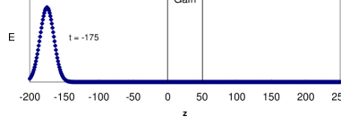
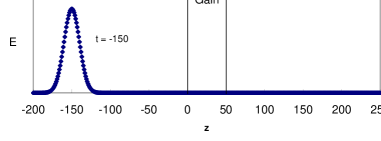
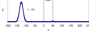
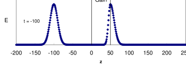
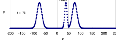
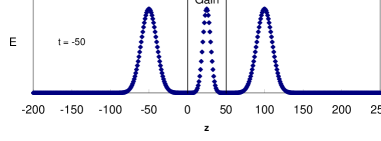
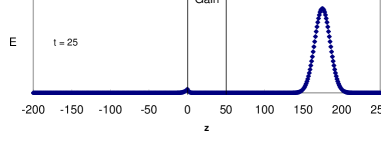
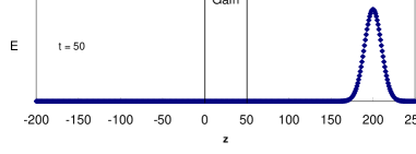
Figure 4: Ten “snapshots” of a Gaussian pulse as it traverses a negative group velocity region $(0<z<50)$, according to eq. (40). The group velocity in the gain medium is $v_{g}=-c/2$, and $c$ has been set to 1.

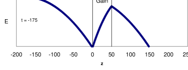
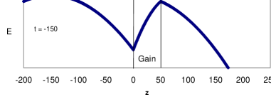
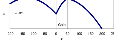
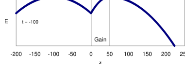
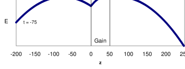
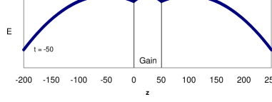
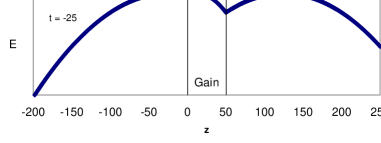
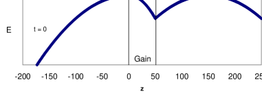
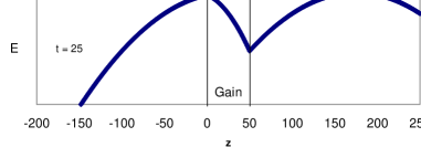
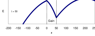
Figure 5: The same as Fig. 4, but with the electric field plotted on a logarithmic scale from 1 to $10^{-65}$.

Our discussion of the pulse has been based on a classical analysis of interference, but, as remarked by Dirac [21], classical optical interference describes the behavior of the wave functions of individual photons, not of interference between photons. Therefore, we expect that the behavior discussed above will soon be demonstrated for a “pulse” consisting of a single photon with a Gaussian wave packet.

The author thanks Lijun Wang for discussions of his experiment, and Alex Granik for references to the early history of negative group velocity and for the analysis contained in eqs. (14)-(16).

References

- [1] L.V. Hau et al., Light speed reduction to 17 metres per second in an ultracold atomic gas, Nature 397, 594-598 (1999).
- [2] K.T. McDonald, Slow light, Am. J. Phys. 68, 293-294 (2000). A figure to be compared with Fig. 1 of the present paper has been added in the version at http://arxiv.org/abs/physics/0007097
- [3] This is in contrast to the “” configuration of the three-level atomic system required for slow light [2] where the pump laser does not produce an inverted population, in which case an adequate classical description is simply to reverse the sign of the damping constant for the pumped oscillator.
- [4] L.J. Wang, A. Kuzmich and A. Dogariu, Gain-assisted superluminal light propagation, Nature 406, 277-279 (2000). Their website, http://www.neci.nj.nec.com/homepages/lwan/gas.htm contains additional material, including an animation much like Fig. 4 of the present paper.
- [5] W.R. Hamilton, Researches respecting vibration, connected with the theory of light, Proc. Roy. Irish Acad. 1, 267, 341 (1839).
- [6] J.S. Russell, Brit. Assoc. Reports (1844), p. 369.
- [7] G.G. Stokes, Problem 11 of the Smith’s Prize examination papers (Feb. 2, 1876), in Mathematical and Physical Papers, Vol. 5 (Johnson Reprint Co., New York, 1966), p. 362.
- [8] T.H. Havelock, The Propagation of Disturbances in Dispersive Media (Cambridge U. Press, Cambridge, 1914).
- [9] H. Lamb, On Group-Velocity, Proc. London Math. Soc. 1, 473-479 (1904).
- [10] See p. 551 of M. Laue, Die Fortpflanzung der Strahlung in dispergierenden und absorbierenden Medien, Ann. Phys. 18, 523-566 (1905).
- [11] L. Mandelstam, Lectures on Optics, Relativity and Quantum Mechanics (Nauka, Moscow, 1972; in Russian).
- [12] L. Brillouin, Wave Propagation and Group Velocity (Academic Press, New York, 1960). That the group velocity can be negative is mentioned on p. 122.
- [13] C.G.B. Garrett and D.E. McCumber, Propagation of a Gaussian Light Pulse through an Anomalous Dispersion Medium, Phys. Rev. A 1, 305-313 (1970).
- [14] R.Y. Chiao, Superluminal (but causal) propagation of wave packets in transparent media with inverted atomic populations, Phys. Rev. A 48, R34-R37 (1993).
- [15] E.L. Bolda, J.C. Garrison and R.Y. Chiao, Optical pulse propagation at negative group velocities due to a nearby gain line, Phys. Rev. A 49, 2938-2947 (1994).
- [16] M.W. Mitchell and R.Y. Chiao, Causality and negative group delays in a simple bandpass amplifier, Am. J. Phys. 68, 14-19 (1998).
- [17] A.M. Steinberg and R.Y. Chiao, Dispersionless, highly superluminal propagation in a medium with a gain doublet, Phys. Rev. A 49, 2071-2075 (1994).
- [18] R.Y. Chiao, Population Inversion and Superluminality, in Amazing Light, ed. by R.Y. Chiao (Springer-Verlag, New York, 1996), pp. 91-108.
- [19] R.Y. Chiao and A.M. Steinberg, Tunneling Times and Superluminality, in Progress in Optics, Vol. 37, ed. by E. Wolf (Elsevier, Amsterdam, 1997), pp. 347-405.
- [20] See p. 943 of R.P. Feynman, A Relativistic Cut-Off for Classical Electrodynamics, Phys. Rev. 74, 939-946 (1948).
- [21] P.A.M. Dirac, The Principles of Quantum Mechanics, 4th ed. (Clarendon Press, Oxford, 1958), sec. 4.