Condensates beyond mean field theory: quantum backreaction as decoherence

Abstract

Abstract    We propose an experiment to measure the slow $\log(N)$ convergence to mean-field theory (MFT) around a dynamical instability. Using a density matrix formalism, we derive equations of motion which go beyond MFT and provide accurate predictions for the quantum break-time. The leading quantum corrections appear as decoherence of the reduced single-particle quantum state.

A Bose-Einstein condensate is described in mean field theory (MFT) by a c-number macroscopic wave function, obeying the Gross-Pitaevskii non-linear Schrödinger equation. MFT is closely analogous to the semiclassical approximation of single-particle quantum mechanics, with the inverse square root of the number $N$ of particles in the condensate playing the role of $\hbar$ as a perturbative parameter. Since in current experimental condensates $N$ is indeed large, it is generally difficult to see qualitatively significant quantum corrections to MFT. In the vicinity of a dynamical instability in MFT, however, quantum corrections appear on timescales that grow only logarithmically with $N$. In this paper we propose an experiment to detect such quantum corrections, and present a simple theory to predict them. We show that, as the Gross-Pitaevskii classical limit of a condensate resembles single-particle quantum mechanics, so the leading quantum corrections appear in the single-particle picture as decoherence.

We will consider a condensate in which particles can only effectively populate two second-quantized modes. This model can be realized with a condensate in a double well potential[1, 2, 3, 4, 5, 6], or with an effectively two-component spinor condensate[7, 8] whose internal state remains uniform in space. Such uniformity can be ensured, to a good approximation, by confining a very cold condensate within a size much smaller than $[n|\sqrt{a_{11}a_{22}}-a_{12}|]^{-1/2}$, where $n$ is the mean total density and $a_{ij}$ is the s-wave scattering length between atoms in internal states $i$ and $j$. The kinetic energy of spin non-uniformity then ensures that the spatial state of the condensate will adiabatically follow its internal state, which will evolve on slower time scales. Dynamical instabilities to phase separation are also frustrated in this regime, which since for available alkali gases all $a_{ij}$ differ only by a few percent, could be reached with small condensates ($N\leq 10^{4}$) in weak, nearly spherical traps ($\omega\leq 100$ Hz). Stronger or less isotropic traps reach the two-mode regime at smaller $N$.

In the double well realization, the nonlinear interaction may be taken to affect only atoms within the same well. In this case single-particle tunneling provides a linear coupling between the two modes, which can in principle be tuned over a wide range of strengths. Two internal states may be coupled by a near-resonant radiation field [9, 10]. If collisions do not change spin states, there is also a simple nonlinear interaction in the internal realization. In either case the total number operator commutes with the Hamiltonian, and may be replaced with the c-number $N$. Discarding c-number terms, we may therefore write the two-mode Hamiltonian

$$H=-\frac{\omega}{2}\left({\hat{a}}_{1}^{\dagger}{\hat{a}}_{2}+{\hat{a}}_{2}^{\dagger}{\hat{a}}_{1}\right)+\frac{\eta}{2}\left[({\hat{a}}_{1}^{\dagger}){\hat{a}}_{1}-({\hat{a}}_{2}^{\dagger}){\hat{a}}_{2}\right]^{2}~{},$$ (1)

where $\omega$ is the coupling strength between the two condensate modes, $\eta$ is the two-body interaction strength, and ${\hat{a}}_{1},{\hat{a}}_{1}^{\dagger},{\hat{a}}_{2},{\hat{a}}_{2}^{\dagger}$ are particle annihilation and creation operators for the two modes. We will take $\eta$ and $\omega$ to be positive, since the relative phase between the two modes may be re-defined arbitrarily, and since without dissipation the overall sign of $H$ is insignificant.

Instead of considering the evolution of ${\hat{a}}_{j}$ and its expectation value in a symmetry-breaking ansatz, we will examine the evolution of the directly observable quantities $\hat{a}_{i}^{\dagger}\hat{a}_{j}$, whose expectation values define the reduced single particle density matrix (SPDM) $R_{ij}\equiv\langle\hat{a}_{i}^{\dagger}\hat{a}_{j}\rangle/N$. It is convenient to introduce the Bloch representation, by defining the angular momentum operators,

$${\hat{L}}_{x}\equiv\frac{{\hat{a}}_{1}^{\dagger}{\hat{a}}_{2}+{\hat{a}}_{2}^{\dagger}{\hat{a}}_{1}}{2}~{},~{}{\hat{L}}_{y}\equiv\frac{{\hat{a}}_{1}^{\dagger}{\hat{a}}_{2}-{\hat{a}}_{2}^{\dagger}{\hat{a}}_{1}}{2i}$$

$${\hat{L}}_{z}=\frac{{\hat{a}}_{1}^{\dagger}{\hat{a}}_{1}-{\hat{a}}_{2}^{\dagger}{\hat{a}}_{2}}{2}~{}.$$ (2)

The Hamiltonian Eq. (1) then assumes the form,

$$H=-\omega{\hat{L}}_{x}+\frac{\eta}{2}\left(\frac{\hat{N}}{4}^{2}+{\hat{L}}_{z}^{2}\right)\;,$$ (3)

and the Heisenberg equations of motion for the three angular momentum operators of Eq. (2) read

$$\frac{d}{dt}{\hat{L}}_{x}=-i[{\hat{L}}_{x},H] = -\frac{\eta}{2}({\hat{L}}_{y}{\hat{L}}_{z}+{\hat{L}}_{z}{\hat{L}}_{y})~{},$$ (4)

$$\frac{d}{dt}{\hat{L}}_{y}=-i[{\hat{L}}_{y},H] = +\omega{\hat{L}}_{z}+\frac{\eta}{2}({\hat{L}}_{x}{\hat{L}}_{z}+{\hat{L}}_{z}{\hat{L}}_{x})~{},$$ (5)

$$\frac{d}{dt}{\hat{L}}_{z}=-i[{\hat{L}}_{z},H] = -\omega{\hat{L}}_{y}~{}.$$ (6)

The mean-field equations for the SPDM in the two-mode model may be obtained, without invoking U(1) symmetry breaking, by approximating second-order expectation values $\langle{\hat{L}}_{i}{\hat{L}}_{j}\rangle$ as products of the first order expectation values $\langle{\hat{L}}_{i}\rangle$ and $\langle{\hat{L}}_{j}\rangle$:

$$\langle{\hat{L}}_{i}{\hat{L}}_{j}\rangle\approx\langle{\hat{L}}_{i}\rangle\langle{\hat{L}}_{j}\rangle~{}.$$ (7)

Defining the single-particle Bloch vector ${\bf{\vec{s}}}=(S_{x},S_{y},S_{z})=(\frac{2\langle{\hat{L}}_{x}\rangle}{N},\frac{2\langle{\hat{L}}_{y}\rangle}{N},\frac{2\langle{\hat{L}}_{z}\rangle}{N}),~{}\kappa=\eta N/2$ and using Eq. (7), we obtain the nonlinear Bloch equations

$${\dot{S}}_{x} = -\kappa S_{z}S_{y}~{},$$ (8)

$${\dot{S}}_{y} = \omega S_{z}+\kappa S_{z}S_{x}~{},$$ (9)

$${\dot{S}}_{z} = -\omega S_{y}~{}.$$ (10)

Mean field trajectories ${\bf{\vec{s}}}(t)$ at four different $\kappa/\omega$ ratios are plotted in Fig. 1. The norm of ${\bf{\vec{s}}}$ is conserved in MFT, and so for an initially pure SPDM, (8) are equivalent to the two-mode Gross-Pitaevskii equation [4].

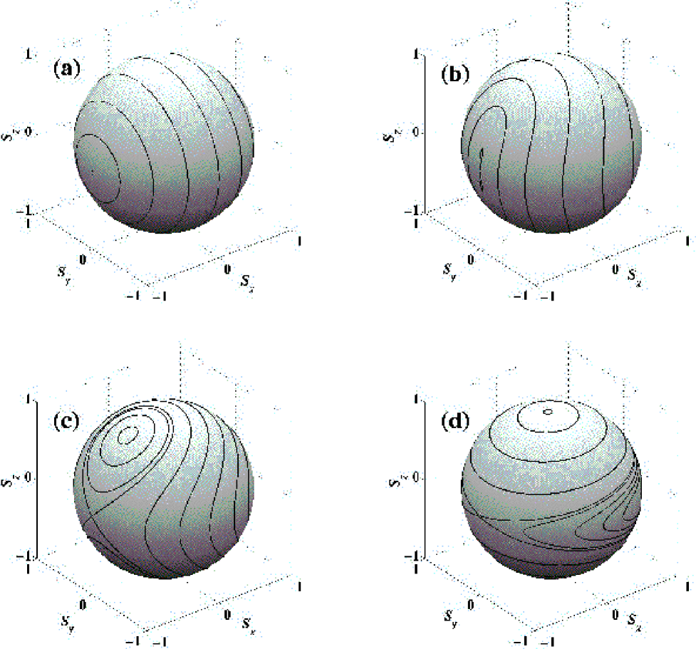
FIG. 1.: Mean-field trajectories at (a)$\kappa=0$, (b)$\kappa=1.02\omega$, (c)$\kappa=2\omega$, and (d)$\kappa=20\omega$.

The nonlinear Bloch equations (8) depict a competition between linear Rabi oscillations in the $S_{y}S_{z}$-plane and nonlinear oscillations in the $S_{x}S_{y}$-plane. For a noninteracting condensate (Fig. 1a) the trajectories on the Bloch sphere are circles about the $S_{x}$ axis, corresponding to harmonic Rabi oscillations. As $\kappa$ increases the oscillations become more anharmonic until, above the critical value $\kappa=\omega$ (Fig. 1b), the stationary point ${\bf{\vec{s}}}=(-1,0,0)$ becomes dynamically unstable, and macroscopic self-trapping can occur (oscillations with a non-vanishing time averaged population imbalance $\langle S_{z}\rangle_{t}\neq 0$) [4]. In the vicinity of the dynamically unstable point, MFT will break down on a time scale only logarithmic in $N$, and so an improved theory is desirable.

If we assume that the condensate remains mildly fragmented, so that the two eigenvalues of $R_{ij}$ are $f$ and $1-f$ for small $f$, we can take ${\hat{L}}_{i}=L_{i}+{\hat{\delta L}}_{i}$, where the c-number $L_{i}$ is ${\cal O}(N)$ and, throughout the Hilbert subspace through which the system will evolve, all matrix elements of $\hat{\delta L}_{i}$ are no greater than ${\cal O}(N\sqrt{f})$. The second order moments

$$\Delta_{ij}=4N^{-2}\left(\langle{\hat{L}}_{i}{\hat{L}}_{j}+{\hat{L}}_{j}{\hat{L}}_{i}\rangle-2\langle{\hat{L}}_{i}\rangle\langle{\hat{L}}_{j}\rangle\right)~{},$$ (11)

will then be of order $f$. We can retain these, and so improve on MFT, if we truncate the BBGKY hierarchy of expectation value equations of motion at one level deeper: we eliminate the approximation (7), and instead impose

$$\langle{\hat{L}}_{i}{\hat{L}}_{j}{\hat{L}}_{k}\rangle\approx\langle{\hat{L}}_{i}{\hat{L}}_{j}\rangle\langle{\hat{L}}_{k}\rangle+\langle{\hat{L}}_{i}\rangle\langle{\hat{L}}_{j}{\hat{L}}_{k}\rangle+\langle{\hat{L}}_{i}{\hat{L}}_{k}\rangle\langle{\hat{L}}_{j}\rangle$$

$$-2\langle{\hat{L}}_{i}\rangle\langle{\hat{L}}_{j}\rangle\langle{\hat{L}}_{k}\rangle\;.$$ (12)

This approximation is accurate to within a factor $1+{\cal O}(f^{3/2})$, better than (7) by one factor of $f^{1/2}$. Successively deeper truncations of the hierarchy yield systematically better approximations as long as $f$ is small.

Applying (11) and (12) to (4), we obtain the following set of equations, in which the mean field Bloch vector drives the fluctuations $\Delta_{ij}$, and is in turn subject to backreaction from them:

$${\dot{S}}_{x} = -\kappa S_{z}S_{y}-\frac{\kappa}{2}\Delta_{yz}$$ (13)

$${\dot{S}}_{y} = \omega S_{z}+\kappa S_{z}S_{x}+\frac{\kappa}{2}\Delta_{xz}$$ (14)

$${\dot{S}}_{z} = -\omega S_{y}$$ (15)

$${\dot{\Delta}}_{xz} = -\omega\Delta_{xy}-\kappa S_{z}\Delta_{yz}-\kappa S_{y}\Delta_{zz}$$ (16)

$${\dot{\Delta}}_{yz} = \omega(\Delta_{zz}-\Delta_{yy})+\kappa S_{z}\Delta_{xz}+\kappa S_{x}\Delta_{zz}$$ (17)

$${\dot{\Delta}}_{xy} = (\omega+\kappa S_{x})\Delta_{xz}-\kappa S_{y}\Delta_{yz}+\kappa S_{z}(\Delta_{xx}-\Delta_{yy})$$ (18)

$${\dot{\Delta}}_{xx} = -2\kappa S_{y}\Delta_{xz}-2\kappa S_{z}\Delta_{xy}$$ (19)

$${\dot{\Delta}}_{yy} = 2(\omega+\kappa S_{x})\Delta_{yz}+2\kappa S_{z}\Delta_{xy}$$ (20)

$${\dot{\Delta}}_{zz} = -2\omega\Delta_{yz}~{}.$$ (21)

In what follows, we will refer to (13) as evolution under ‘Bogoliubov backreaction’ (BBR).

We note that (13) are actually identical to the equations of motion one would obtain, for the same quantities, using the Hartree-Fock-Bogoliubov Gaussian ansatz. And if the second-order moments $\Delta_{ij}$ may initially be factorized as $\Delta_{ij}=\delta_{i}\delta_{j}$ ($i,j=x,y,z$), then the factorization persists and the time evolution of $\delta_{x},\delta_{y}$, and $\delta_{z}$ is equivalent to that of perturbations of the mean-field equations (8):

$${\dot{\delta}}_{x} = -\kappa(S_{z}\delta_{y}+S_{y}\delta_{z})~{},$$ (22)

$${\dot{\delta}}_{y} = \omega\delta_{z}+\kappa(S_{z}\delta_{x}+S_{x}\delta_{z})~{},$$ (23)

$${\dot{\delta}}_{z} = -\omega\delta_{y}~{}.$$ (24)

Thus our equations for $\Delta_{ij}$ are in a sense equivalent to the usual Bogoliubov equations. The quantitative advantage of our approach therefore lies entirely in the wider range of initial conditions that it admits, which may more accurately represent the exact initial conditions. For instance, a Gaussian approximation will have $\Delta_{xx}={\cal O}(1)$ in the ground state, where in fact $\Delta_{xx}={\cal O}(N^{-1})$. This leads to an error of order $N^{-1/2}$ in the Josephson frequency computed by linearizing (13) around the ground state, which is problematic because one would hope that the Gaussian backreaction result would be accurate at this order. Our SPDM approach avoids this problem, which is presumably the two-mode analogue of the Hartree-Fock-Bogoliubov spectral gap[11].

For finite motion of the Bloch vector, our formalism offers an efficient method to depict the back-reaction of the Bogoliubov equations on the mean field equations via the coupling terms $-\kappa\Delta_{yz}/2$ and $\kappa\Delta_{xz}/2$ in (13). Because in general $\Delta_{yz}(t)\neq\Delta_{xz}(t)$, this back-reaction has the effect of breaking the unitarity of the mean-field dynamics. Consequently, the BBR trajectories are no longer confined to the surface of the Bloch sphere, but penetrate to the interior (representing mixed-state $R_{ij}$, with two non-zero eigenvalues). Thus although decoherence is generally considered as suppressing quantum effects, decoherence of the single particle quantum state of a condensate is itself the leading quantum correction (due to interparticle entanglement) to the effectively classical MFT.

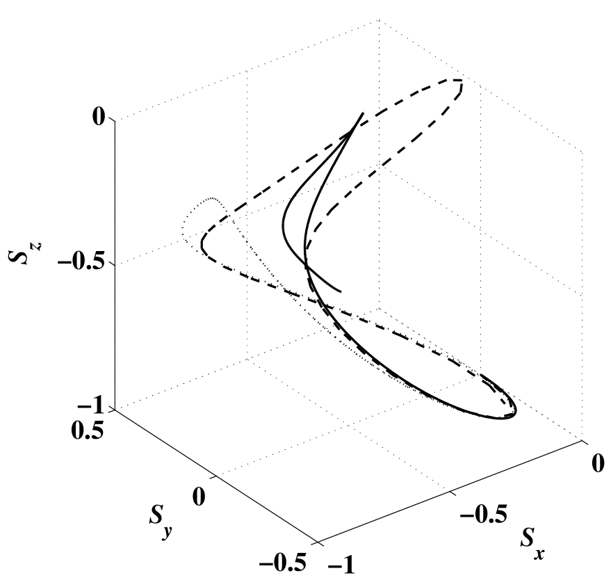
FIG. 2.: Mean field ($\cdot\cdot\cdot$), Bogoliubov back-reaction ($---$) and exact 50 particles (—–) trajectories starting with all particles in one mode, at $\kappa=2\omega$.

In order to confirm this decoherence, and demonstrate how the BBR equations (13) improve on the mean-field equations (8), we compare the trajectories obtained by these two formalisms to exact quantum trajectories, obtained by fixing the total number of particles $N=50$ and solving Eq. (4) numerically, using a Runge-Kutta algorithm. The results for an initial state where all particles are in one of the modes (corresponding to the initial conditions $S_{x}=S_{y}=0,S_{z}=-1,\Delta_{xx}=-\Delta_{yy}=2/N,\Delta_{xy}=\Delta_{xz}=\Delta_{yz}=\Delta_{zz}=0$) and $\kappa=2\omega$ are shown in Fig. 2. The MFT trajectory passes through the dynamically unstable point ${\bf{\vec{s}}}=(-1,0,0)$. Consequently, the quantum trajectory sharply breaks away from the MFT trajectory as it approaches this point, entering the Bloch sphere interior. While still periodic on a much shorter time scale than the exact evolution, the BBR evolution (dashed curve) provides an excellent prediction of the time at which the break from MFT takes place (the ’quantum break time’).

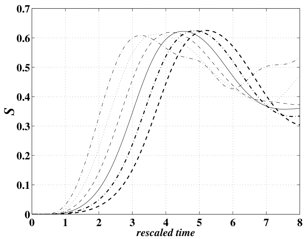
FIG. 3.: Growth of the von Neumann entropy $S$ of the quantum reduced single-particle density operator, at $\kappa=2\omega$, for N=10 ($-\cdot-$), 20 ($\cdot\cdot\cdot$), 40 ($---$), 80 (——), 160 (- . - . -), and 320 (- - - -) particles. Initial conditions are the same as in Fig. 2.

The quantum break time near a dynamical instability is expected to grow logarithmically with N. In Fig. 3 we plot the von Neumann entropy

$$S=-\frac{1}{2}\ln\left[\frac{(1+|{\bf{\vec{s}}}|)^{(1+|{\bf{\vec{s}}}|)}(1-|{\bf{\vec{s}}}|)^{(1-|{\bf{\vec{s}}}|)}}{4}\right]$$ (25)

of the exact reduced single-particle density operator, as a function of the rescaled time $\omega t$ with N=10,20,40,80,160, and 320 particles, for the same initial conditions as in Fig. 2. Since the MFT entropy is always zero, $S$ serves as a measure of convergence. The quantum break time is clearly evident, and indeed increases as $\log(N)$. The single-particle entropy is measurable, in the internal state realization of our model, by applying a fast Rabi pulse and measuring the amplitude of the ensuing Rabi oscillations, which is proportional to the Bloch vector length $|{\bf{\vec{s}}}|$. (Successive measurements with Rabi rotations about different axes, i.e. by two resonant pulses differing by a phase of $\pi/2$, will control for the dependence on the angle of ${\bf{\vec{s}}}$). In a double well realization, one could determine the single-particle entropy by lowering the potential barrier, at a moment when the populations on each side were predicted to be equal, to let the two parts of the condensate interfere. The fringe visibility would then be proportional to $|{\bf{\vec{s}}}|$. Since $|{\bf{\vec{s}}}|$ at a fixed time depends exponentially on $\eta$, such experiments could also potentially be used to measure scattering lengths.

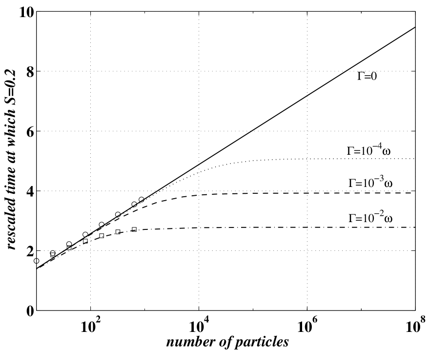
FIG. 4.: Time at which $S$ reaches 0.2 as a function of the particle number $N$, according to the BBR equations (13), modified to include thermal phase-diffusion. Four different values of $\Gamma$ are shown: $\Gamma=0$ (—–), $\Gamma=10^{-4}\omega$ ($\cdot\cdot\cdot$), $\Gamma=10^{-3}\omega$ ($---$), and $\Gamma=10^{-2}\omega$ ($-\cdot-$). Exact quantum results are presented for $\Gamma=0$ (circles) and $\Gamma=10^{-2}\omega$ (squares). Initial conditions, $\kappa$ and $\omega$ are the same as in Figs. 2 and 3.

Decoherence of quantum systems coupled to reservoirs shows similar behaviour to Fig. (3). The entropy of a dynamically unstable quantum system coupled to a reservoir[12], or of a stable system coupled to a dynamically unstable reservoir, is predicted to grow linearly with time, at a rate independent of the system-reservoir coupling, after an onset time proportional to the logarithm of the coupling. This shows that one can really consider the Bogoliubov fluctuations as a reservoir [13], coupled to the mean field with a strength proportional to $1/N$. But one can also consider decoherence due to a genuine reservoir (unobserved degrees of freedom, as opposed to unobserved higher moments). For example, thermal particles scattering off the condensate mean field will cause phase diffusion[14] at a rate $\Gamma$ which may be estimated in quantum kinetic theory as proportional to the thermal cloud temperature. For internal states not entangled with the condensate spatial state, $\Gamma$ may be as low as $10^{-5}$ Hz under the coldest experimental conditions, whereas for a double well the rate may reach $10^{-1}$ Hz. Further sources of decoherence may be described phenomenologically with a larger $\Gamma$. Evolving the full $N$-particle density matrix under the appropriate quantum kinetic master equation [3], we again solve for ${\bf{\vec{s}}}$ either numerically or in BBR approximation. In Fig. 4 we show the time at which the entropy reaches a given value, as a function of the number of particles, for various $\Gamma$, according to the modified BBR equations. The exact quantum results (limited by computation power to $N\sim 10^{3}$) are presented for the two limiting values of $\Gamma$, showing excellent agreement with the BBR predictions. These results can of course be interpreted as a quantum saturation of the dephasing rate at low temperature.

This work was partially supported by the National Science Foundation through a grant for the Institute for Theoretical Atomic and Molecular Physics at Harvard University and Smithsonian Astrophysical Observatory.

REFERENCES

- [1] J. Javanainen, Phys. Rev. Lett. 57, 3164 (1986); J. Javanainen and S. Yoo, Phys. Rev. Lett. 76, 161 (1996).
- [2] M. Jack, M. Collett, and D. Walls, Phys. Rev. A 54, R4625 (1996); G. J. Milburn, J. Corney, E. M. Wright, D. F. Walls, Phys. Rev. A 55, 4318 (1997); A. S. Parkins and D. F. Walls Phys. Rep. 303, 1 (1998).
- [3] J. Ruostekoski and D. F. Walls, Phys. Rev. A 58, R50 (1998).
- [4] A. Smerzi, S. Fantoni, S. Giovanazzi, and S. R. Shenoy, Phys. Rev. Lett. 79, 4950 (1997); S. Raghavan, A. Smerzi, S. Fantoni, and S. R. Shenoy, Phys. Rev. A 59, 620 (1999); I. Marino, S. Raghavan, S. Fantoni, S. R. Shenoy, and A. Smerzi, Phys. Rev. A 60, 487 (1999).
- [5] I. Zapata, F. Sols, and A. Leggett, Phys. Rev. A 57, R28 (1998).
- [6] P. Villain and M. Lewenstein, Phys. Rev. A 59, 2250 (1999).
- [7] M. R. Matthews, B. P. Anderson, P. C. Haljan, D. S. Hall, M. J. Holland, J. E. Williams, C. E. Wieman, and E. A. Cornell, Phys. Rev. Lett. 83, 3358 (1999).
- [8] C. J. Myatt, E. A. Burt, R. W. Ghrist, E. A. Cornell, and C. E. Wieman, Phys. Rev. Lett. 78, 586 (1997).
- [9] M. R. Matthews, D. S. Hall, D. S. Jin, J. R. Ensher, C. E. Wiemann, E. A. Cornell, F. Dalfovo, C. Minniti, and S. Stringari, Phys. Rev. Lett. 81, 243 (1998); J. Williams, R. Walser, J. Cooper, E. Cornell, and M. Holland, Phys. Rev. A 59, R31 (1999).
- [10] Patrik Öhberg and Stig Stenholm, Phys. Rev. A 59, 3890 (1999).
- [11] A. Griffin, Phys. Rev. B 53, 9341 (1996).
- [12] J.-P. Paz and W.H. Zurek, Phys. Rev. Lett. 72, 2508 (1994).
- [13] S. Habib, Y. Kluger, E. Mottola, and J.-P. Paz, Phys Rev Lett 76, 4660 (1996).
- [14] J.R. Anglin, Phys. Rev. Lett. 79, 6 (1997).