Equations for Stochastic Macromolecular Mechanics of

Single Proteins: Equilibrium Fluctuations, Transient

Kinetics and Nonequilibrium Steady-State

Hong Qian

Department of Applied Mathematics

University of Washington, Seattle, WA 98195, U.S.A.

(206)-543-2584 (Phone), (206)-685-1440 (Fax)

qian@amath.washington.edu

ABSTRACT

A modeling framework for the internal conformational dynamics and external mechanical movement of single biological macromolecules in aqueous solution at constant temperature is developed. Both the internal dynamics and external movement are stochastic; the former is represented by a master equation for a set of discrete states, and the latter is described by a continuous Smoluchowski equation. Combining these two equations into one, a comprehensive theory for the Brownian dynamics and statistical thermodynamics of single macromolecules arises. This approach is shown to have wide applications. It is applied to protein-ligand dissociation under external force, unfolding of polyglobular proteins under extension, movement along linear tracks of motor proteins against load, and enzyme catalysis by single fluctuating proteins. As a generalization of the classic polymer theory, the dynamic equation is capable of characterizing a single macromolecule in aqueous solution, in probabilistic terms, (1) its thermodynamic equilibrium with fluctuations, (2) transient relaxation kinetics, and most importantly and novel (3) nonequilibrium steady-state with heat dissipation. A reversibility condition which guarantees an equilibrium solution and its thermodynamic stability is established, an H-theorem like inequality for irreversibility is obtained, and a rule for thermodynamic consistency in chemically pumped nonequilibrium steady-state is given.
Keywords: free energy, nano-biochemistry, Smoluchowski equation, stochastic process, thermal fluctuation

I. Introduction

Progress in optics, electronics, and computer science has now made it possible to study biological macromolecules in aqueous solution at constant temperature by observing experimentally and measuring quantitatively the behavior of single biological macromolecules. These studies have been providing and will continue to yield important information on the behavior and properties of individual biomolecules and to reveal molecular interactions in and the mechanisms of biological processes. The impact which single-molecule studies will have on molecular biology may be gauged by comparison with the pioneering studies on single channel proteins in membranes, which have revolutionized physiology.¹ The highly quantitative data obtained in these novel measurements, with piconewton and nanometer precision on the forces and movements of single macromolecules, complement those from traditional kinetic studies and structural determinations at the atomic level.

The novel experimental approach requires a consistent theoretical framework for quantitatively understanding, interpreting, and integrating laboratory data.^2-6 The objective is to develop a unifying molecular theory, with thermodynamic consistency, which is capable of integrating the three classes of quantitative measurements on macromolecules: macroscopic (spectroscopic kinetics), mesoscopic (single molecules), and microscopic (atomic structures). In this paper, we show how the spectroscopically defined kinetics, expressed in terms of discrete conformational states, is integrated with the mechanics of a macromolecule. The philosophy behind this approach, Stochastic Macromolecular Mechanics, is that we realize the impracticality of representing the entire conformational space of a macromolecule with a high-dimensional energy function. Hence we still rely on a discrete-state Markov model with experimentally defined “states” and kinetic parameters. However, we introduce a continuous energy landscape when there are relevant, mechanical data on the single molecule. Therefore the stochastic macromolecular mechanics is a mix of the discrete-state Markov kinetics with Brownian dynamics based on available and relevant experimental measurements. It is a mesoscopic theory with a single set of equations. The theoretical approach helps researchers to identify the relevant (random) variables and key parameters in a macromolecular system or process, and provides them with the necessary equations.

The discrete-state master equation approach has been long accepted as the natural mathematical description for biochemical kinetics of individual molecules.^7,8 With more detailed information on molecular structures and energetics, the Smoluchowski’s continuous description of overdamped Brownian dynamics has found numerous applications in condensed matter physics, polymer chemistry, and biochemistry of macromolecules^9,10. Hänggi et al.¹¹ have reviewed the related work with Kramers’ approach to chemical rate theory in which the assumption on overdamping is not warranted. However, for biological macromolecules in aqueous solution, and with the time scale of biological interests, this assumption is generally acceptable. In dealing with a single protein molecule, the discrete approach is appropriate for spectroscopic studies³ while the continuous approach is necessary for mechanical measurements. By combining these two descriptions, the stochastic macromolecular mechanics treats the internal conformational dynamics of proteins as well as its external mechanics. In particular, both internal and external forces are explicitly considered. On the mathematical side, such a combination leads to coupled stochastic processes,¹² giving rise to three different classes of problems: reversible stationary processes (in a physicist’s term, thermal equilibrium with fluctuations), nonstationary processes (kinetic transient), and irreversible stationary processes (nonequilibrium steady-state with dissipation). The last class of processes is novel^13-15 and necessary for modeling motor protein (e.g. kinesin and myosin) movement and energetics,^16-26 as well as other “active macromolecules”.

The differential equations in stochastic macromolecular mechanics are Fokker-Planck-master type (linear diffusion-convection equations with variable coefficients) based on conservation of probability.⁸ This type of equations is different from the well-studied nonlinear reaction-diffusion equations ^27,28 with distinctly different mathematical properties.^15,21

We would like to point out that there is already a large literature on both Smoluchowski equation and master equations. The novelty of our formalism is that (i) in order to combine the two types of equation into one, a condition analogous to the “thermodynamic box” in the elementary chemical kinetics needs to be introduced. This relation, called potential condition,²⁹ yields a constraint between the energy functions in the Smoluchowski equation and the transition rates in the master equation. This constraint guarantees the time-reversibility of the stationary solution to the stochastic macromolecular mechanics (SM₃), similar to that of fluctuation-dissipation relation required in modeling equilibrium Brownian motion. More importantly, however, is that (ii) for single macromolecules like motor proteins, this condition is violated due to the presence of chemical pumping (i.e., ATP hydrolysis).^21,22 This latter class of models based on Smoluchowski-master equation is relatively new. Its relation to the phenomena of stochastic resonance has been revealed only recently.^30,31 And finally, (iii) the stationary solution to the SM₃ with chemical pumping defines a nonequilibrium steady-state the thermodynamics of which can be rigorously investigated. By thermodynamics, we mean the entropy production, heat dissipation, nonlinear irreversible force-flux relationship, and the law of thermodynamics. It is this third aspect of the SM₃, we suggest, makes the Smoluchowski approach more powerful and fundamental than that is generally aware. SM₃ as a statistical thermodynamic theory for macromolecules in isothermal aqueous solution, both passive and active, will have wide applications, and deserves further investigations in the light of single-molecule experiments.

A second objective of this paper is introducing the physical chemists who are interested in the Smoluchowski’s approach to the unique and exciting opportunity in the current biophysics of nonequilibrium macromolecules on the level of single molecules. In that sense, SM₃ is a generalization of the classic polymer theory⁹ into the nonlinear (Sec. II) and nonequilibrium (Sec. III) regime.

The paper is organized with increasing complexity as follows. In Sec. II we show how external force is introduced into the kinetics of protein-ligand dissociation. We point out that mechanical measurements on single molecular complex depend critically on the experimental conditions - the stiffness of the force probe and the rate of its retraction. In Sec. III, polymers consisting of nonlinear subunits are introduced and we show how the internal kinetics is coupled to the external mechanics and movement. A Boltzmann’s H-theorem like inequality is obtained; and the importance of nonlinear spring in serial leading to complex mechanical behavior is discussed. Sec. IV introduces the ATP hydrolysis into the model. Detailed balance, nonequilibrium steady-state, and thermodynamic consistency are discussed. Sec. V. shows how SM₃ can be applied to the well-studied problem of fluctuating enzyme and yields new insights. In particular, we show how the classic concepts such as thermodynamic linkage and induced fit are consequence of the detailed balance, and can be generalized and quantified. A summary is given in Sec. VI.

II. Macromolecular Mechanics of Protein-Ligand Dissociation

In this section, we discuss the dissociation of a single protein-ligand complex under an external force introduced by an experimenter.^32-34 As in any mechanics measurement, one first is interested in the position of the ligand with respect to the center of the mass of the protein. The next mechnical quantity is what is the forces acting on the ligand. This leads to a Newtonian equation in which one neglects the acceleration term

$$\beta\frac{dx}{dt}=F_{int}(x)+F_{ext}(x,t)+f(t).$$ (1)

The four terms are $(i)$ frictional force with frictional coefficient $\beta$, $(ii)$ intermolecular force between the ligand and the protein, with potential energy function $U_{int}(x)$: $F_{int}(x)$=$-dU_{int}(x)/dx$, $(iii)$ the external force, and $(iv)$ the stationary, pure random force due to collisions between the ligand and the solvent molecules: $\langle f(t)\rangle=0$. Because of the presence of the random force $f(t)$, the movement $x(t)$ is stochastic, e.g., it is a Brownian motion. Mathematically equivalent, the Smoluchowski’s description of overdamped Brownian dynamics is based on a partial differential equation of parabolic type:^29,35

$$\beta\frac{\partial P(x,t)}{\partial t}=k_{B}T\frac{\partial^{2}P(x,t)}{\partial x^{2}}-\frac{\partial}{\partial x}\left[(F_{int}(x)+F_{ext}(x,t))P(x,t)\right]$$ (2)

where $P(x,t)$ is now the probability density of the ligand being at $x$ at time $t$. $k_{B}$ is the Boltzmann constant, and $T$ is temperature which characterizes the magnitude of the random force $f(t)$: $\langle f(t)f(t^{\prime})\rangle=2k_{B}T\delta(t-t^{\prime})$.

The above Eq. (1) and (2) lay the mathematical basis for all models, but the choices for $U_{int}(x)$ and $F_{ext}$ set the difference between different models. In the work of Shapiro and Qian,^36-38 $U_{int}=V_{0}[(x_{0}/x)^{12}-2(x_{0}/x)^{6}]$ with a smooth repulsive force, and $F_{ext}=k(x-d(t))$ where $k$ is the stiffness of the force probe exerting the external force, and $d(t)=vt$ is the position of the piezoelectric motor which drives the force probe, $v$ is the retracting velocity. In the work of Evans and Ritchie,^39,40 $U_{int}=-V_{0}(x_{0}/x)^{n}$ $(x>x_{0})$ with an abrupt repulsion at $x_{0}$, and $F_{ext}=-F(t)$ is independent of $x$. These differences give qualitatively similar but qualitative different results. Hence they can be quantitatively tested against experimental date.

Fig. 1 shows the results of simulations on the force-displacement curve for a protein-ligand complex with a simple 6-12 Lennard-Jones potential, measured using an elastic force probe. It is important to note that all the differences between the curves are due to the difference in the stiffness of the force probe ($k$), the rate of retraction ($v$), and the temperature ($k_{B}T$) at which the measurements are carried out. Therefore, this calculation demonstrates that the “raw” experimental data can only be understood, in general, in terms of a molecular model. It is important to realize the significance of the measurement aparatus on the experimental data.

III. Macromolecular Mechanics of Polyglobular Protein Unfolding

In the previous section on protein-ligand dissociation, we have completely neglected the conformational change within the protein itself. The protein was treated as a rigid body exerting a force on the ligand. A more realistic model must consider the possibility of the protein’s internal conformational change due to the external force, acting via the ligand. In this section, we study the unfolding of a polyglobular protein under extensional force. This problem naturally involves the internal dynamics of the macromolecules.

To be concrete, let’s consider the recent experimental work on giant muscle protein titin.^41-43 Titin is a protein with many globular domains (subunits) in serial. The subunits unfold under an external force pulling the entire molecule. The folded state of each subunit is rigid, and the unfolded state of each subunit can be regarded as a coiled polymer spring. Hence the conformational state of the entire protein, to a first order approximation, can be characterized by $n$: the number of unfolded subunits within the molecule. Let’s assume the total number of subunits are $N$, and let $x$ be the total extension of the titin molecule (along the axis of external force), then a realistic characterization of a titin molecule is by two dynamic variables $(x,n)$, $(x\geq 0,\ 0\leq n\leq N)$.

The equation of motion for $x$ is again

$$\beta\frac{dx}{dt}=-\frac{dU_{int}(x,n)}{dx}+F_{ext}+f(t)$$ (3)

in which $n$ is itself a random (discrete-state Markov) process. Hence the above equation is coupled to a master equation

$$\frac{\partial P(n,t)}{\partial t}=(N-n+1)\lambda_{u}(x,n-1)P(n-1,t)+(n+1)\lambda_{f}(x,n+1)P(x,n+1,t)$$

$$-[n\lambda_{f}(x,n)+(N-n)\lambda_{u}(x,n)]P(n,t)$$ (4)

where $P(n,t)$ is the probability for $n$ at time $t$. $\lambda_{f}$ and $\lambda_{u}$ are folding and unfolding rate constants of individual subunits. They are functions of the force acting on the subunit, which in turn is determined by the total extension of the molecule ($x$) and the number of unfolded domains in the chain ($n$).

A comprehensive description of both the internal dynamics and external movement can be obtained by combining Eq. (3) and (4). We therefore have

$$\frac{\partial P(x,n,t)}{\partial t} = \left(\frac{k_{B}T}{\beta}\right)\frac{\partial^{2}P(x,n,t)}{\partial x^{2}}+\frac{1}{\beta}\frac{\partial}{\partial x}\left[\left(\frac{dU_{int}(x,n)}{dx}+F_{ext}\right)P(x,n,t)\right]$$ (5)

$$+ (N-n+1)\lambda_{u}(x,n-1)P(x,n-1,t)$$

$$+ (n+1)\lambda_{f}(x,n+1)P(x,n+1,t)$$

$$- [n\lambda_{f}(x,n)+(N-n)\lambda_{u}(x,n)]P(x,n,t)$$

where $P(x,n,t)$ is the joint probability distribution of the titin molecule having internally $n$ unfolded domains and external extension $x$.

As in the previous section, particular models will provide specific $\lambda_{f}(x,n)$, $\lambda_{u}(x,n)$, and $U_{int}(x,n)$. These functions are not totally independent, however. Microscopic reversibility dictates that

$$\frac{\lambda_{u}(x,n)}{\lambda_{f}(x,n+1)}=\frac{n+1}{N-n}\exp\left[-\frac{U_{int}(x,n+1)-U_{int}(x,n)}{k_{B}T}\right].$$ (6)

This condition guarantees that the stationary solution to Eq. (5) is a thermodynamic equilibrium with time reversibility. Furthermore, this reversibility condition (also known as potential condition and detailed balance) also guarantees the thermodynamic stability of the equilibrium state in terms of a generalized free energy function. As we shall see below, without (6), the stationary solution in general represents a nonequilibrium steady-state with dissipation.

With the reversibility condition and in the absence of external force $F_{ext}$, it is easy to verify that the stationary solution to Eq. (5) is

$$P^{*}(x,n)=Z^{-1}e^{-U(x,n)/k_{B}T}$$ (7)

where

$$Z=\sum_{n=0}^{N}\int_{0}^{\infty}e^{-U(x,n)/k_{B}T}.$$

The time-dependent solutions to (5) are dynamic models for nonstationary transient kinetics of macromolecules.

We now show that the equilibrium solution $P^{*}(x,n)$ is asymptotically stable. By stability, we mean a molecule approaches to its equilibrium state irrespective of its initial state. We introduce a free energy functional:

$$\Psi[P(x,n,t)] = \sum_{n=0}^{N}\int_{0}^{\infty}\left(U(x,n)P(x,n,t)+k_{B}TP(x,n,t)\ln P(x,n,t)\right)dx$$

$$= -k_{B}T\ln Z+k_{B}T\sum_{n=0}^{N}\int_{0}^{\infty}P(x,n,t)\ln\left(\frac{P(x,n,t)}{P^{*}(x,n)}\right)dx$$

in which the second term (known as relative entropy^44,45) is always nonnegative and equal to zero if and only if $P(x,n,t)=P^{*}(x,n)$.²⁹ Based on Eq. (5) the time derivative of $\Psi$ is

$$\dot{\Psi}[P(x,n,t)]=-\sum_{n=0}^{N}\int_{0}^{\infty}\left[\beta^{-1}J^{2}(x,t)P^{-1}+k_{B}T\left(J_{n}^{+}-J_{n}^{-}\right)\ln\left(\frac{J_{n}^{+}}{J_{n}^{-}}\right)\right]dx\leq 0$$ (8)

where

$$J(x,t)=-k_{B}T\frac{\partial P(x,n,t)}{\partial x}-\frac{dU(x,n)}{dx}P(x,n,t)$$

and

$$J_{n}^{+}(t)=(n+1)\lambda_{f}(x,n+1)P(x,n+1,t),\hskip 8.5359ptJ_{n}^{-}(t)=(N-n)\lambda_{u}(x,n)P(x,n,t).$$

The integrand in Eq. (8) is always positive. Hence $\Psi$ is a Lyapunov functional for the time-dependent solution of Eq. (5), which guarantees $P^{*}$ to be asymptotically stable. Furthermore, because of the reversibility condition, the differential equation in (5) is symmetric and all its eigenvalues are real, indicating relaxations in such systems can not oscillate.

The physical interpretation of the above result is important: It relates the equation of SM₃ to the second law of thermodynamics. The $\Psi$-function is the generalization of the equilibrium free energy of a closed, isothermal molecular system. $\Psi$ decreases monotonically to its minimum $-k_{B}T\ln Z$, the Gibbs free energy, when the system reaches its equilibrium. It is intriguing to note that the dynamics in Eq. (5) is not governed by the gradient of the free energy. Nevertheless, one should see the analogy between Eq. (8) and the H-theorem of Boltzmann in his approach to irreversibility in an isolated system (microcanonical ensemble).

To analyze the stochastic dynamics of a complex macromolecule under extensional force, it is important first to have an essential understanding of its nonlinear mechanical property. A polyglobular protein model is a generalization of the classic “bead-and-spring” to nonlinear spring.⁹ The protein subunits all have two energy minima while a simple Hookean spring has only one. This leads to fundamentally different behavior of the macromolecule. To illustrate this, let’s apply the elementary Ohm’s law for nonlinear springs in serial: the force on the springs are the same while the displacement is additive. For simplicity, assume each subunit has a potential function (and force) given in Fig. 2. This energy function has been used in recent work on globular protein folding kinetics. Then Fig. 3 gives a quantitative force-extension curve expected from a polyglobular protein with three subunits. As one can see, the most striking feature is the possibility of multiple branches of the curve with a given force. This is due to the combinatorics shown in Table I.

IV. Macromolecular Mechanics of Motor Protein Movement

With the presence of the reversibility (potential) condition, the previous model represents a “passive” complex molecule. Without the external force, such molecules relax, multi-exponentially, to a thermodynamic equilibrium. They are biochemically interesting, but they are not “alive”. One could argue that one of the fundamental properties of a living organism is the ability to convert energy among different forms (solar to electrical, electrical to chemical, chemical to mechanical, etc.). We now show how stochastic macromolecular mechanics can be used to develop models for chemomechanical energy transduction^16,17 in single motor proteins.⁴⁶ In the absence of an external force, a motor protein is undergoing nonequilibrium steady-state with ATP hydrolysis and generating heat – representing a rudimentary form of energy metabolism.

The key for developing a theory for motor protein is to consider that while biochemical studies of a protein in test tubes probe a set of discrete conformational states of the molecule, the mechanical studies of a protein measure positions and forces. Internally, a motor protein has many different conformational states within a hydrolysis cycle, and a reaction scheme usually can be deduced from various kinetic studies. While the protein is going through its conformational cycles, its center of mass moves along its designated linear track (e.g., kinesin on a microtubule, myosin on an actin filament, and polymerase on DNA) which usually has a periodic structure. The movement is stochastic; the interaction between the motor and the track (the force field) are usually different for different internal states of the molecule.

These basic facts lead to the following equation

$$\frac{\partial P(x,n,t)}{\partial t} = \left(\frac{k_{B}T}{\beta}\right)\frac{\partial^{2}P(x,n,t)}{\partial x^{2}}+\frac{1}{\beta}\frac{\partial}{\partial x}\left[\left(\frac{dU_{int}(x,n)}{dx}+F_{ext}\right)P(x,n,t)\right]$$ (9)

$$+ \sum_{k=1}^{N}\left[\lambda_{kn}(x)P(x,k,t)-\lambda_{nk}(x)P(x,n,t)\right],$$

where $P(x,n,t)$ denote the joint probability of a motor protein with internal state $n$ and external position $x$. $U_{int}(x,n)$ is the interaction energy between the protein in state $n$ and the track. $\lambda_{\ell m}(x)$ is the transition rate constant from internal state $\ell$ to state $m$ when the protein is located at $x$. Some of the $\lambda$’s are pseudo-first order rate constants which contain the concentrations [ATP], [ADP], and [Pi].

When the ratio [ADP][Pi]/[ATP] = $K_{eq}$, the equilibrium constant for the hydrolysis reaction, the $U(x,n)$ and $\lambda_{\ell m}^{*}(x)$ are again constrained by the reversibility (the superscript ^∗ is to indicate that the pseudo-first order rate constants are calculated in terms of the equilibrium concentrations):

$$\frac{\lambda_{\ell m}^{*}(x)}{\lambda_{m\ell}^{*}(x)}=\exp\left(-\frac{U_{int}(x,m)-U_{int}(x,\ell)}{k_{B}T}\right).$$ (10)

This relation was called “thermodynamic-consistency” by T. L. Hill⁴⁷ in his landmark contribution to the Huxley’s theory of muscle contraction⁴⁸. It has to be satisfied by every motor protein models. It is clear, however, that the ATP, ADP, and Pi can be kept at arbitrary values. Hence in general the stationary solution of the Eq. (9) will be a nonequilibrium steady-state. Sustaining the concentrations is a form of “pumping” which keeps the system at nonequilibrium steady-state³¹ with positive entropy production and heat generation.^14,15 Such a molecular device is also known as isothermal ratchet.^18,19,22 See Ref. 21 and 15 for reviews of the vast literature. If the concentrations are not actively sustained, then they will change slowly (since there is only a single molecule at work hydrolyzing ATP) and eventually reach a thermal equilibrium state in which (10) is satisfied.

As in the previous sections, a practical model requires specific choices for the parameters $U$ and $\lambda$. In the past several years, a large amount of work have appeared on modeling translational motor proteins such as myosin and kinesin^{15,18,19,21,25,21} and rotational motor proteins such as ATP synthase.^49,50 A thermodynamically valid model for a motor protein has to satisfy Eq. (10) when [ADP][Pi]/[ATP] = $K_{eq}$, but in general without a potential function. This rule has not been enforced in some of the models.

Simpler but phenomenological models based on discrete-state kinetics have also been developed for motor protein kinetics and energetics.^20,23-25 It is important to point out that these models are completely in accord with the present continuous theory. However, drastic simplifications are used in order to make the models more accessible to experimental data. Fig. 4 shows the conceptual relationship between these two classes of models. Therefore, the discrete model should not be viewed as an alternative to the SM₃, rather it is a simplification which can be further scrutinized in terms of the general theory of SM₃. The stistical thermodynamics associated with the continuous approach, however, can be developed in parallel for the discrete models.²⁵

V. Macromolecular Mechanics of Fluctuating Enzyme

Equilibrium conformational fluctuation of proteins play an important role in enzyme kinetics. The theory of fluctuating enzyme⁵¹ can be developed naturally in terms of the above equations for stochastic macromolecular mechanics. Let’s consider a single enzyme, with its internal conformation characterized by $x$, and $N$ number of substrate molecules. The enzyme catalyzes a reversible isomerization reaction between two forms of the substrate (reactant and product), with rate constants $\lambda_{+}(x)$ and $\lambda_{-}(x)$.

The equation for the catalytic reaction coupled with the enzyme conformational fluctuation, according to stochastic macromolecular mechanics, is

$$\frac{\partial P(n,x,t)}{\partial t}=-[n\lambda_{+}+(N-n)\lambda_{-}]P(n,x,t)+(n+1)\lambda_{+}P(n+1,x,t)$$

$$+(N-n+1)\lambda_{-}P(n-1,x,t)+D\frac{\partial^{2}P(n,x,t)}{\partial x^{2}}+k\frac{\partial}{\partial x}(xP(n,x,t)),\hskip 8.5359pt$$ (11)

$$(0\leq n\leq N)$$

where $P(n,x,t)$ is the probability of at time $t$ having $n$ number of reactant molecules and the enzyme internal conformation being at $x$. $D$ and $k$ characterize the protein conformational fluctuation. $x$ is perpendicular to the isomerization reaction coordinate as first proposed by Agmon and Hopfield,¹⁰ in contrast to the other models which address random energy landscape along the reaction coordinate.⁵² Eq. (11), which is essentially the same equation for the modeling of polyglobular protein unfolding (Eq. 5), unifies and generalizes most of the important works on fluctuating enzymes.

Along this approach, most work in the past have addressed the non-stationary, time-dependent solution to (11). These studies are motivated by macroscopic experiments which are initiated ($t=0$) with all the substrate in only the reactant form. If $\lambda_{-}(x)=0$ and $N=1$, Eq. (11) is reduced to that of Agmon and Hopfield.¹⁰ If $\lambda_{-}(x)=0$ but $N$ is large, then one can introduce a continuous variable $\xi=n/N$, known as the survival probability, and Eq. (11) can be approximated as (see Appendix I for more discussion)

$$\frac{\partial P(\xi,x,t)}{\partial t}=\lambda_{+}(x)\frac{\partial}{\partial\xi}(\xi P(\xi,x,t))+D\frac{\partial^{2}P(\xi,x,t)}{\partial x^{2}}+k\frac{\partial}{\partial x}(xP(\xi,x,t)).$$ (12)

At $t=0$, Prob$\{\xi=1\}=1$.

The moments of $\xi$, $\langle\xi^{m}\rangle(x,t)=\int_{0}^{1}\xi^{m}P(\xi,x,t)d\xi$, can be easily obtained from Eq. (12):

$$\frac{\partial\langle\xi^{m}\rangle}{\partial t}=-m\lambda_{+}(x)\langle\xi^{m}\rangle+D\frac{\partial^{2}\langle\xi^{m}\rangle}{\partial x^{2}}+k\frac{\partial}{\partial x}\left(x\langle\xi^{m}\rangle\right).$$ (13)

Note Eq. (11) with $N=1$ and Eq. (13) for $\langle\xi\rangle$ are idential. For $\lambda_{+}(x)=\alpha x^{2}+\beta x+\gamma$, Eq. (13) can be exactly solved by various methods if one realizes that its solution has a Gaussian form^53-55 (also see Appendix II). From Eq. (13) one immediately sees that high-order moments $\langle\xi^{m}\rangle$ is related to $\langle\xi\rangle$ by $\lambda_{+}(x)\rightarrow m\lambda_{+}(x)$.⁵⁶

Different choices for $\lambda_{+}(x)$ lead to quantitatively different models for fluctuating enzymes in the literature. $\lambda_{+}(x)\propto e^{-\alpha x}$ represents a fluctuating activation energy barrier;¹⁰ $\lambda_{+}(x)=\alpha(x+\overline{x})$ $(>0)$ representing a fluctuating cofactor concentration;⁵⁷ $\lambda_{+}(x)$ = $\alpha x^{2}$ representing a fluctuating geometric bottleneck.⁵³

We now consider the reversible reaction (with $\lambda_{-}(x)\neq 0$) which has not been discussed previously. This class of models is more appropriate for recent measurements in single-molecule enzymology.³ Again we assume $N$ being large. Hence we have

$$\frac{\partial P(\xi,x,t)}{\partial t}=\frac{\partial}{\partial\xi}\left(D_{\xi}(\xi,x)\frac{\partial P(\xi,x,t)}{\partial\xi}\right)+\frac{\partial}{\partial\xi}\left(V_{\xi}(\xi,x)P(\xi,x,t)\right)$$

$$+D\frac{\partial^{2}P(\xi,x,t)}{\partial x^{2}}+\frac{\partial}{\partial x}(V_{x}(x,\xi)P(\xi,x,t))$$ (14)

where $D_{\xi}(\xi,x)=[\xi\lambda_{+}+(1-\xi)\lambda_{-}]/2N$ and $V_{\xi}=\xi\lambda_{+}-(1-\xi)\lambda_{-}$. Eq. (14) is a 2D diffusion-convection equation similar to a continuous model we proposed for motor protein movement.²¹ One important consequence of this formulation and the reversibility condition is realizing that conformational fluctuations of the enzyme, $V_{x}$ can not be independent of the substrate. This constitutes the essential idea of induced fit^58-60 and thermodynamic linkage!^61,57 For equilibrium fluctuation, again reversibility (i.e., potential condition) dictates:²¹

$$\frac{\partial V_{x}(x,\xi)}{\partial\xi}=D\frac{\partial}{\partial x}\left(\frac{V_{\xi}(\xi,x)}{D_{\xi}(\xi,x)}\right)=\frac{4ND(\lambda_{-}\lambda_{+}^{\prime}-\lambda_{+}\lambda_{-}^{\prime})\xi(1-\xi)}{[\xi\lambda_{+}+(1-\xi)\lambda_{-}]^{2}}$$ (15)

where $\lambda^{\prime}=d\lambda(x)/dx$. Therefore,

$$V_{x}(x,\xi)=-\frac{\xi}{(\lambda_{+}-\lambda_{-})^{2}}+\frac{\lambda_{+}+\lambda_{-}}{(\lambda_{+}-\lambda_{-})^{3}}\ln[\lambda_{+}\xi+\lambda_{-}(1-\xi)]$$

$$+\frac{\lambda_{+}\lambda_{-}}{(\lambda_{+}-\lambda_{-})^{3}[\lambda_{+}\xi+\lambda_{-}(1-\xi)]}+V_{0}(x)$$ (16)

where $V_{0}(x)$ is an arbitrary function of $x$ but it is independent of $\xi$. As can be seen, if $\lambda_{-}<<\lambda_{+}$, then there is no requirement for $\xi$-dependent $V_{x}$.

VI. Conclusions

Biological macromolecules are the cornerstone of molecular biology. Mathematical modeling of biomolecular processes requires a comprehensive and thermodynamically consistent theoretical basis upon which quantitative analyses can be carried out and rigorously compared with experiments. In this paper, a formal theory, we call stochastic macromolecular mechanics, is presented. The theory offers a dynamic equation for describing the internal kinetics as well as external motion of macromolecules in aqueous solution at constant temperature. Systematically applying this theory to various biomolecular processes will bring molecular biophysics closer to the standard of theoretical chemistry and physics. At present time, Smoluchowski is well-known for its importance in calculating the microscopic fluctuations of an isothermal equilibrium system.^8,9,29,35 It is less known that it can also be a cogent model for a macromolecules under chemical pumping.^18,19,30,21 What has not been appreciated is that this mesoscopic model also yields equilibrium and nonequilibrium thermodynamics for the macromolecule. Therefore, it deserves the same status as that of Newton’s for mechanics, Navier-Stokes’ for fluid dynamics, Maxwell’s for electrodynamics, Schrödinger’s for quantum mechanics, and Boltzmann’s for statistical mechanics of isolated systems.

Acknowledgement

I like to dedicate this paper to Professor Joel Keizer. Officially I have not worked with him. However, he had been a mentor to me in the past 10 years because our common interests in nonequilibrium statistical mechanics and biophysics, and because of Terrell Hill. One can easily find his influence on my work presented here. He will be sorely missed.

Appendix I

Let’s use the well-known linear death process⁶² as an example to illustrate the continuous approximation for the discrete model:

$$\frac{dP_{n}(t)}{dt}=-n\lambda P_{n}(t)+(n+1)\lambda P_{n+1}(t)$$ (17)

where $P_{n}(t)$ is the probability of survival population being $n$ at time $t$. The solution to this equation is well known⁶²

$$P_{n}(t)=\frac{N!}{n!(N-n)!}e^{-n\lambda t}\left(1-e^{-\lambda t}\right)^{N-n}$$

where $N$ is the total population at time $t=0$. It is easy to show that the moments

$$\langle n(t)\rangle = Ne^{-\lambda t},$$

$$\frac{\langle n^{2}(t)\rangle}{\langle n(t)\rangle^{2}} = 1+\frac{1}{N}\left(e^{\lambda t}-1\right),$$ (18)

$$\frac{\langle n^{3}(t)\rangle}{\langle n(t)\rangle^{3}} = 1+\frac{3(N-1)}{N^{2}}\left(e^{\lambda t}-1\right)+\frac{1}{N^{2}}\left(e^{2\lambda t}-1\right).$$

We now consider the continuous counterpart of (17) with $\xi=n/N$:

$$\frac{\partial P(\xi,t)}{\partial t}=\frac{\partial}{\partial\xi}\left(\xi P(\xi,t)\right)$$

which has solution

$$P(\xi,t)=e^{\lambda t}\delta\left(\xi e^{\lambda t}-1\right)$$

for initial condition $P(\xi,0)=\delta(\xi-1)$. The moments for $\xi$ are

$$\langle\xi^{k}(t)\rangle=e^{-k\lambda t}.$$ (19)

Comparing (18) and (19), we note that the continuous approximation is valid when the $N$ is large and $t$ is small. More precisely, $\ln N\gg\lambda t$.

Appendix II

Let’s consider the following equation

$$\frac{\partial u}{\partial t}=D\frac{\partial^{2}u}{\partial x^{2}}+k\frac{\partial}{\partial x}(xu)-(\alpha x^{2}+\beta x+\gamma)u$$

In Gaussian form⁵³ which is equivalent to path integral calculation⁵⁴ $u(x,t)$ = $[2\pi\sigma(t)]^{-1/2}$ $\exp\left\{\nu(t)-[x-\mu(t)]^{2}/2\sigma^{2}(t)\right\}$, and equate coefficients of like order terms in $x$ we have

$$d\nu/dt = -\alpha[\mu^{2}(t)+\sigma^{2}(t)]-\beta\mu(t)-\gamma$$

$$d\mu/dt = -[k+2\alpha\sigma^{2}(t)]\mu(t)-\beta\sigma^{2}(t)$$

$$d\sigma^{2}/dt = 2D-2k\sigma^{2}(t)-2\alpha\sigma^{4}(t)$$

with initial condition $\sigma^{2}(0)=D/k$, $\mu(0)=0$, and $\nu(0)=0$. We thus have

$$\sigma^{2}(t) = 2D\frac{(\omega+k)+(\omega-k)e^{-2\omega t}}{(\omega+k)^{2}-(\omega-k)^{2}e^{-2\omega t}}$$

$$\mu(t) = \left(\frac{2\beta D}{\omega}\right)\frac{-1+e^{-\omega t}}{(\omega+k)-(\omega-k)e^{-\omega t}}$$

$$\nu(t) = \left(\frac{\beta^{2}D}{\omega^{2}}-\frac{\omega-k}{2}-\gamma\right)t+\frac{4\beta^{2}D}{\omega(\omega-k)}\left[\frac{1}{(\omega+k)-(\omega-k)e^{-\omega t}}-\frac{1}{2k}\right]$$

$$\hskip 115.63243pt-\frac{1}{2}\ln\left[\frac{(\omega+k)^{2}-(\omega-k)^{2}e^{-2\omega t}}{4\omega k}\right]$$

where $\omega^{2}=k^{2}+4D\alpha$.

References

¹ B. Sakmann and E. Neher, Single-channel recording, 2nd Ed. (Plenum Press, New York, 1995)

² X. S. Xie, and J. K. Trautman, Ann. Rev. Phys. Chem. 49, 441 (1998).

³ X. S. Xie and H. P. Lu, J. Biol. Chem. 274, 15967 (1999).

⁴ H. Qian and E. L. Elson, Biophys. J. 76, 1598 (1999).

⁵ H. Qian, Biophys. J. 79 137 (2000).

⁶ H. Qian, J. Math. Biol. 41, 331 (2000).

⁷ D. A. McQuarrie, J. Appl. Prob. 4, 413 (1967).

⁸ J. Keizer, Statistical Thermodynamics of Nonequilibrium Processes (Springer-Verlag, New York, 1987).

⁹ M. Doi and S. F. Edwards, The Theory of Polymer Dynamics (Clarendon, Oxford, 1986).

¹⁰ N. Agmon, and J. J. Hopfield, J. Chem. Phys. 78, 6947 (1983).

¹¹ P. Hänggi, P. Talkner, and M. Borkovec, Rev. Mod. Phys. 62, 251 (1990).

¹² M. Qian, and B. Zhang, Acta Math. Appl. Sinica 1, 168 (1984).

¹³ M.-P. Qian, M. Qian, and G. L. Gong, Contemp. Math. 118, 255 (1991).

¹⁴ H. Qian, Proc. R. Soc. Lond. A. , in the press (2001).

¹⁵ H. Qian, J. Math. Chem. 27, 37 (2000).

¹⁶ T. L. Hill, Free Energy Transduction in Biology (Academic Press, New York, 1977).

¹⁷ T. L. Hill, Free Energy Transduction and Biochemical Cycle Kinetics (Springer-Verlag, New York, 1989).

¹⁸ C.S. Peskin, G.B. Ermentrout, and G.F. Oster, in Cell Mechanics and Cellular Engineering, edited by V.C. Mow, F., Guilak, R. Tran-Son-Tay, and R. M. Hochmuth (Springer-Verlag, New York, 1994), pp. 479-489.

¹⁹ R.D. Astumian, Science 276, 917 (1997).

²⁰ H. Qian, Biophys. Chem. 67, 263 (1997).

²¹ F. Jülicher, A., Ajdari, and J. Prost, Rev. Mod. Phys. 69, 1269 (1997).

²² H. Qian, Phys. Rev. Lett. 81, 3063 (1998).

²³ M. E. Fisher and A. B. Kolomeisky, Proc. Natl. Acad. Sci. USA 96, 6597 (1999).

²⁴ M. E. Fisher and A. B. Kolomeisky, Physica A 274, 241 (1999).

²⁵ H. Qian, Biophys. Chem. 83, 35 (2000).

²⁶ D. Keller and C. Bustamante, Biophys. J. 78, 541 (2000).

²⁷ J. D. Murray, Mathematical Biology, 2nd, corrected Ed. (Springer-Verlag, New York, 1993).

²⁸ H. Qian, and J.D. Murray, App. Math. Lett. 14, 405 (2001).

²⁹ H. Risken, The Fokker-Planck Equation: Methods of Solution and Applications (Springer-Verlag, New York, 1984).

³⁰ L. Gammaitoni, P. Hänggi, P. Jung, and F. Marchesoni, Rev. Mod. Phys. 70, 223 (1998).

³¹ H. Qian and M. Qian, Phys. Rev. Lett. 84, 2271 (2000).

³² E. Florin, V. T. Moy, and H. E. Gaub, Science 264, 415 (1994).

³³ V. T. Moy, E. Florin, and H. E. Gaub, Science 266, 257 (1994).

³⁴ A. Chilkoti, T. Boland, R. D. Ratner, and P. S. Stayton, Biophys. J. 69, 2125 (1995).

³⁵ N. G. van Kampen, Stochastic Processes in Physics and Chemistry, Revised and enlarged Ed. (North-Holland, Amsterdam, 1997).

³⁶ B. E. Shapiro and H. Qian, Biophys. Chem. 67, 211 (1997).

³⁷ B. E. Shapiro and H. Qian, J. Theoret. Biol. 194, 551 (1998).

³⁸ H. Qian and B. E. Shapiro, Prot: Struct. Funct. Genet. 37, 576-581 (1999).

³⁹ E. Evans and K. Richie, Biophys. J. 72, 1541 (1997).

⁴⁰ E. Evans and K. Richie, Biophys. J. 76, 2439 (1999).

⁴¹ M. S. Z. Kellermayer, S. B. Smith, H. L. Granzier, and C. Bustamante, Science 276, 1112 (1997).

⁴² M. Rief, M. Gautel, F. Oesterhelt, J. M. Fernandez, and H. E. Gaub, Science 276, 1109 (1997).

⁴³ L. Tskhovrebova, J. Trinick, J. A. Sleep, and R. M. Simmons, Nature 387, 308 (1997).

⁴⁴ M. C. Mackey, Rev. Mod. Phys. 61, 981 (1989).

⁴⁵ H. Qian, Phys. Rev. E. in the press.

⁴⁶ J. Howard, Ann. Rev. Physiol. 58, 703 (1996).

⁴⁷ T. L. Hill, Progr. Biophys. Mol. Biol. 28, 267 (1974).

⁴⁸ A. F. Huxley, Progr. Biophys. 7, 255 (1957).

⁴⁹ T. Elston, H.Y. Wang, and G. Oster, Nature 391, 510 (1998)

⁵⁰ H.Y. Wang, and G. Oster, Nature 396, 279 (1998).

⁵¹ C. Blomberg, J. Mol. Liquids 42, 1 (1989).

⁵² R. Zwanzig, Proc. Natl. Acad. Sci. USA, 85, 2029 (1988).

⁵³ R. Zwanzig, J. Chem. Phys. 97, 3587 (1992).

⁵⁴ J. Wang and P.G. Wolynes, Chem. Phys. Lett. 212, 427 (1993).

⁵⁵ J. Wang and P.G. Wolynes, Chem. Phys. 180, 141 (1994).

⁵⁶ J. Wang and P.G. Wolynes, Phys. Rev. Lett. 74, 4317 (1995).

⁵⁷ E. Di Cera, J. Chem. Phys. 95, 5082 (1991).

⁵⁸ D. E. Koshland, Proc. Natl. Acad. Sci. USA 44, 98 (1958).

⁵⁹ H. Qian and J. J. Hopfield, J. Chem. Phys. 105, 9292 (1996).

⁶⁰ H. Qian, J. Chem. Phys. 109, 10015 (1998).

⁶¹ J. Wyman, J. Mol. Biol. 11, 631 (1965).

⁶² H. M. Taylor and S. Karlin,An Introduction to Stochastic Modeling, 3rd Ed. (Academic Press, San Diego, 1998).

⁶³ R. Zwanzig, Proc. Natl. Acad. Sci. U.S.A. 92, 9801 (1995).

⁶⁴ R. Doyle, K.T. Simon, H. Qian, and D. Baker, Prot: Struct. Funct. Genet. 29, 282 (1997).

⁶⁵ H. Qian and S.I. Chan, J. Mol. Biol. 286, 607 (1999).

Figure Captions

Figure 1. The force-displacement curve for a simple Lennard-Jones bond calculated based on the solution of stochastic dynamics Eq. (2). The $F_{int}=1/x^{7}-1/x^{13}$ which equals zero when $x=1$, and $F_{ext}(x)=k(x-vt-1)$. The ordinate is $\langle F\rangle$ = $\int_{0}^{\infty}F_{ext}(x)P(x,t)dx$, and the abscissa is $\langle x\rangle$. The line labeled LJ is the expected Lennard-Jones force. As one can see, with increasing temperature, decreasing retracting rate, and stiffer probe, the measured force-displacement curve approaches to the LJ curve. It is also noted that with small $k_{B}T$, there is a mechanical “bond rupturing”^36,38, while at larger $k_{B}T$, the maximal force can be significantly smaller than that of LJ due thermally activated transtion.

Figure 2. (A) A conceptual energy landscape for a globular protein, cooperative folding^63-65 (not to the appropriate scale) with a transition state at $x^{{\ddagger}}$. For a single domain of titin, the reasonable $x_{o}=10\AA$ and $L=30nm$. The folded state is represented by the deep energy well and unfolded (random coil) state is represented by a shallow well with large entropy. The reaction coordinate (the abscissa) is uniquely defined by the direction of the mechanical force which pulls the molecule. At very small $x$, there is a closely packed core of all the atoms in the domain. Large $x$ asymptotically approaches the contour length $L$ of the polypeptide chain:

$$E(x)=\alpha\left\{\frac{V_{0}}{x_{o}}\left[-2\left(\frac{x_{o}}{x}\right)^{6}+\left(\frac{x_{o}}{x}\right)^{12}\right]\right\}-\beta x+\gamma\left[\frac{k_{B}TL}{\ell_{p}(1-x/L)}\right]$$

where $x_{o}$ is the size of folded protein, $V_{0}$ is the energy of the folded state, and $\ell_{p}$ is the persistence length of the polypeptide random coil. $\alpha$, $\beta$ and $\gamma$ are parameters characterizing folded, unfolded, and stretched states of the molecule. In the figure they are chosen as $\alpha V_{0}/x_{o}=20$, $\beta=1$, and $\gamma k_{B}TL/\ell_{p}=1$, and $L=10$. (B) The corresponding force as function of displacement, $F_{1}(x)=dE(x)/dx$. $I$, $II$, and $III$ are used to label the three monotonic regions of the curve. Note region $II$ including the transition state is mechanically unstable.

Figure 3. The force-extension relation for a series of three globular domains each of which is characterized by Fig. 2B. The integers by the curves are labels for the branches in the curve. For three subunits in serial, the force is the same on different subunits and the total extension is the sum of the three individual extensions. Each branch is a sum of three from the $I$, $II$, and $III$ in Fig. 2B. Therefore, there are total 27 branches for a trimer, but only 10 are distinguishable (see Table I). Any branch involves $II$ (dotted lines) is mechanically unstable. The stable branches are 1, 5, 8, 10. The dashed lines with the slope $-k$ represent the force-displacement for the elastic force probe with stiffness $k$.^36,38 The bold sawtooth curve⁴² is expected from a mechanical force-extension experiment. A measurement using a force probe with less stiffness and slower rate will show less of the sawtooth pattern.

Figure 4. $x$ = $n-1$, $n$, $n+1$, … in the figure represent the periodic binding sites of a motor protein along its track. $A$, $B$ and $C$ are the chemical states of the motor protein, i.e., the cyclic hydrolysis reaction can be written as $A\rightleftharpoons B\rightleftharpoons C\rightleftharpoons A$. If the potential energy $U_{int}(x,k)$ is such that the motor can move along the track only simultaneously when $B\longrightarrow C$, and there is well-defined energy barriers between $x=n$ and $x=n+1$ for $A$, $B$, and $C$, then we have a simplified discrete model (line with bold face) for the stochastic kinetics of a motor protein. One of the most important consequences of these assumptions is that the ATP hydrolysis and the motor protein stepping are tightly coupled.²⁵

Table I

curve # 1 2 3 4 5 6 7 8 9 10 composition I,I,I I,I,II I,II,II II,II,II I,I,III I,II,III II,II,III I,III,III II,III,III III,III,III multiplicity 1 3 3 1 3 6 3 3 3 1

Table Caption

Table I Each branch in Fig. 3 consists of a sum of 3 terms in Fig. 2B: $I$, $II$, and $III$ (Colume 2). There are total 27 branches, but some of them overlap and Colume 3 shows the multiplicity.

Figure 1:

Figure 2:

Figure 3:

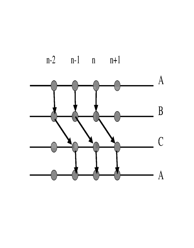
Figure 4: