Remote sensing of bubble clouds in seawater

Abstract

We report on the influence of submerged bubble clouds on the remote sensing properties of water. We show that the optical effect of bubbles on radiative transfer and on the estimate of the ocean color is significant. We present a global map of the volume fraction of air in water derived from daily wind speed data. This map, together with the parameterization of the microphysical properties, shows the possible significance of bubble clouds on the albedo of incoming solar energy.

Keyword: Remote sensing reflectance, Bubble clouds, Radiative transfer

1 Introduction

“The effect of bubbles on the color of the sea may be observed in breaking waves… Where a great many bubbles have been entrained by a breaking wave it is white. But where there are fewer of them it is blue-green or green, brighter than the sea but not as bright as the foamiest parts of the wave. Even after a wave has broken and the water is again quiescent, a pastel green patch often remains, slowly fading into the surrounding sea as the bubbles dissipate. Thus the effect of bubbles on the color of the sea is similar to that of solid particles (Bohren, 1987).” Bubbles within the water and foam on its surface (Bukata, 1995; Frouin et al., 1996; Stramski, 1994) can predominate in determining the radiative transfer properties of the sea surface at higher wind speeds. However, there is a limited knowledge about the radiative transfer properties of bubble clouds, their inherent optical properties (IOP), and their global climatology. Mobley (1994) and Bukata (1995) discuss qualitatively the surface properties of bubble clouds. Frouin et al. (1996) performed spectral reflectance measurements of sea foam at the Scripps Institution of Oceanography Pier. They observed a decrease of the foam reflectance in the near-infrared and proposed that the foam reflectance can not be decoupled from the refelectance by bubbles. Stramski (1994) concentrates on light scattering by submerged bubbles in quiescent seas and shows the scattering coefficient and the backscattering coefficient at 550 nm in comparison with scattering and backscattering coefficients of sea water as estimated from the chlorophyll-based bio-optical models for Case 1 waters. In this exploratory paper, we report on the influence of bubble clouds generated by breaking waves on the remote sensing reflectance and calculate not only the inherent optical, but also apparent optical properties using the radiative transfer model. We show that the optical effects of bubbles on remote sensing of the ocean color are significant. Furthermore, we present a global map of volume fraction of air in water. This map, together with the parameterization of the microphysical properties, shows the significance of bubble clouds on the global albedo of incoming solar energy. By proxy, we show the influence of the bubble clouds on the remote sensing retrieval of organic and inorganic components of the natural waters. It is worth mentioning that the bubble clouds coincide with the upper range of the euphotic zone and will, therefore, contribute to the dynamics of the upper-ocean boundary layer, heat distribution, and sea surface temperature (Thorpe et al., 1992). In fact, our initial motivation for this work was an observation that the asymptotic radiance distribution is established close to the ocean surface in apparent contradiction with theoretical studies (Flatau et al., 1999). Thus, the light field must become diffuse at shallower depths than usually modeled. This leads to search for alternative mechanisms influencing the light distribution. Thus, the importance to light scattering of the bubble clouds goes beyond the remote sensing issues considered in this work.

In the next section, we discuss in more detail the microphysical and morphological properties of bubble clouds, because they have a direct bearing on their optical properties and radiative transfer.

2 Physical properties of bubble clouds

2.1 Morphology of bubble clouds in natural waters

Individual bubble clouds are generated by breaking waves, persist for several minutes (Thorpe, 1995), and reach to mean depths of about $4H_{s}$, where $H_{s}$ is the significant wave height, but with some clouds extending to about $6H_{s}$. There is evidence that at high wind speeds, separate bubble clouds near the surface coalesce, producing a stratus layer (Thorpe, 1995). Fig 1 is based on a sonograph of Thorpe (1984). The “bubble-stratocumulus” (b-Sc) is often observed by acoustic means (Farmer and Lemon, 1984; Thorpe, 1995). The depth of the b-Sc layer is related to the wind speed and wind variability, but more specifically it is set by larger waves, such us those breaking predominantly in groups (Thorpe, 1995). The “stratus layer” description should not be taken too literally. For sufficiently high winds there will be significant concentrations through out the upper layer, but the variability within this layer can be very high.

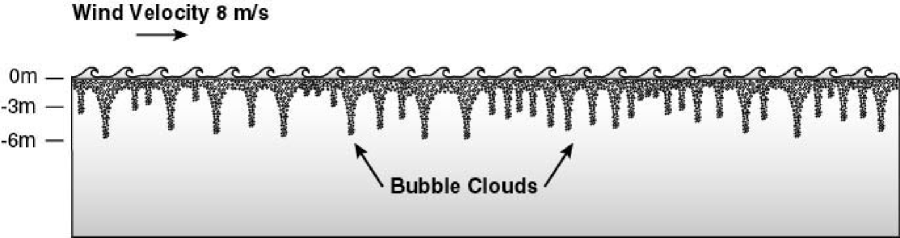
Figure 1: Bubble-stratocumulus (b-Sc) layer generated by breaking waves with inhomogeneous deeper intrusions. The depth of the cloud is related to the maximum significant wave height.

2.2 Bubble cloud climatology

According to Thorpe et al. (1992) in the absence of precipitation and in wind speeds exceeding about 3 m s^-1, wave breaking generally provides the dominant source of bubbles. The wind speed $W_{10}$ at 10 m above the mean sea surface level is used to parameterize the volume fraction of air in water, $f=V_{\rm air}/V_{w}$, where $V_{\rm air}$ is the volume of air, and $V_{w}$ is the volume of water. This parameterization is an approximation of a more complex wind-wave relationship.

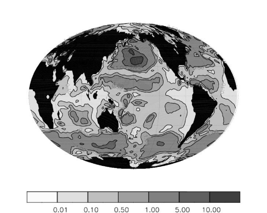
Figure 2: January 1992, monthly averaged volume fraction. Volume fraction $\times 10^{6}$.

Figure 2 shows the volume fraction of air in water estimated from the $W_{10}$ winds for January of 1992. The volume fraction and the wind speed are assumed to follow a non-linear relationship (Walsh and Mulhearn, 1987)

$$f=f_{0}W_{10}^{4.4}+f_{1}$$ (1)

The coefficients $f_{0}$ and $f_{1}$ were calculated at 2m assuming that f= $10^{-8}$ for $W_{10}=6.2{\rm m\;s^{-1}}$ and f= $10^{-7}$ for $W_{10}=10.5{\rm m\;s^{-1}}$ (Walsh and Mulhearn, 1987). Vagle and Farmer (1992) show that the volume fraction decreases with depth, changing from about $10^{-6}$ at 0.3 m to $10^{-7}$ at 2.7 m. We base our parameterization on these findings and extrapolate (1) to near-sea-surface depth using exponential fit.

The monthly averages of $f$ were obtained by employing 1992 daily surface winds from the NCAR/NCEP (Kalnay et al., 1996) reanalysis project, and averaging the daily volume fractions for each month. Thus, Figure 2 is based on the variability of the wind field on the scale of one day. In the winter of the northern hemisphere, one can observe maxima associated with the midlatitude storm tracks in the Northern Pacific. Cyclogenesis, common in western parts of the oceans during the winter, contributes to mixing and a large bubble cloud volume fraction. This can be observed to the east of the North American continent. The Intertropical Convergence Zone (ITCZ) region, with its associated deep convection, may also be a region of enhanced production of bubbles. The winds of the Southern Ocean have a strong effect on bubble formation during both summer and winter. In subtropical regions, to the west of the continents, the subsidence associated with the descending branch of the Hadley circulation is responsible for the relative minimum in $f$. It should be stressed that these results are qualitative and that they can be improved by more detailed breaking wave climatology models (Kraus and Businger, 1994). The data in Fig 2 is indicative of regions where bubble clouds are potentially important in the interpretation of remotely sensed reflectance.

2.3 Optical thickness

The size distribution of bubble clouds determines the optical thickness and is, therefore, one of the most critical parameters entering the theory. There are two assumptions which simplify the development here: (a) we consider light scattering in the geometric optics regime for which the ratio proportional to bubble radius to wavelength $x=2\pi r/\lambda$ is large and (b) we assume that there is an effective radius $r_{\rm eff}$ which determines the optical properties of the size distribution. Both (a) and (b) are quite probable. The size parameter, $x=50$, corresponding to a bubble radius of approximately 5 ${\rm\mu m}$, is already in the geometric optics regime, and $r_{\rm eff}=10{\rm\mu m}$ will satisfy (a). For bubbles with an effective radius of $r_{\rm eff}$, the volume attenuation (equal to scattering for a non-absorbing sphere) can be expressed as

$$b=Q_{\rm sca}{N\over V_{w}}s=2{V_{\rm air}\over V_{w}}{N\over V_{\rm air}}s=2f{s\over v}.$$ (2)

Thus

$$b=2{f\over r_{\rm eff}}$$ (3)

where $s=\pi r^{2}$ is the cross-section of a bubble with radius $r$, $v$ is the volume of such a bubble. $N$ is the number of bubbles in volume $V_{w}$ of water and $f$ is the fraction of air in a volume of water. The effective radius is defined as $r_{\rm eff}=v/s$ (Stephens et al., 1990; King et al., 1993; Bricaud and Morel, 1986). Scattering efficiency defines how much of incoming light is being “blocked” by a particle by scattering processes, for large size parameters $Q_{\rm sca}$ tends to 2. This issue is discussed in detail by Bohren and Huffman (1983).

The physical significance of $f$ comes from the fact that it is determined by the large scale forcing such as the wind field. Thus, for a given synoptic or climatological setting, the mixing ratio $f$ is, to some extent, pre-determined. On the other hand, the effective radius $r_{\rm eff}$ depends on processes of much smaller scale then the large scale. These processes are coagulation, coalescence, coating by organic material, saturation, buoyancy, pressure, etc. Thus, Eq. 3 defines the optical properties of bubble clouds on both the large- and sub-scales. The expression $b=2f/r_{\rm eff}$ holds for polydispersions, and the only difference with a monodispersion is that $r_{\rm eff}$ is defined via distribution averaged $s$ and $v$.

2.4 Effective radius of the size distribution

Numerous observations of bubble size distributions are reported in the literature based on acoustic, photographic, optical, and holographic methods (Wu, 1988a). Akulichev and Bulanov (1987) summarize results from 22 experiments using different techniques. As the origins of bubbles are biological (within the volume and at the bottom), as well as physical (at the rough surface), we may expect large regional and temporal variations of bubble concentration between coastal and open oceanic waters and between plankton bloom or no-bloom conditions (Thorpe et al., 1992).

Figure 3 presents a comparison of bubble spectra under breaking waves and quiescent sea. Recently published observations, using laser holography near the ocean surface, have shown that the densities of 10 to 15$\mu$m radius bubbles can be as high as $10^{6}$ (per cubic meter per micron radius increment) within 3 m of the surface of quiescent seas (O’Hern et al., 1988). These results are plotted as solid squares connected with a vertical solid line. The majority of bubbles injected into the surface layers of natural waters is unstable, either dissolving due to enhanced surface tension and hydrostatic pressures or rising to the air-water interface where the bubbles break (Johnson and Wangersky, 1987). However, bubbles with long residence times, i.e. stable microbubbles, have been observed. For example Medwin (1977) observed nearly $2.5\times 10^{6}$of bubbles per cubic meter in the radius range $18-355$ $\mu$m for small wind speeds. One of the stabilization mechanisms (Mulhearn, 1981; Johnson and Wangersky, 1987) assumes that the surfactant material is a natural degradation product of chlorophyll, present in almost all photosynthesizing algae. Isao et al. (1990) have observed very large populations of neutrally buoyant particles with radii between $0.1-1\mu$m. Johnson and Wangersky (1987) and Thorpe et al. (1992) proposed another stabilization mechanism based on monolayers of adsorbed particles. Numerical modeling (Thorpe et al., 1992) can be used to study the effects of water temperature, dissolved gas saturation levels, and particulate concentrations on the size distribution of subsurface bubbles. The results of such numerical models provide additional evidence for the existence of a small size bubble fraction which is not adequately measured by acoustic or photographic techniques. The dashed line on Fig. 3 presents the mean concentration in the model steady-state for the water temperature of 0C. It can be seen that maximum concentration is around $15\mu$m and it is 2.5 orders of magnitude larger than for 100$\mu$m bubbles. Other results presented (Figure 3) are those of Johnson and Cooke (1979) observations at 4m in wind speed 11-13${\rm m\;s}^{-1}$ (open squares). In situ acoustic measurements of microbubbles at sea by Medwin (1977) are plotted as solid triangles. The solid triangles joined by a solid line are concentrations at 4m depth and 3.3m$s^{-1}$ wind speed. These spectra were obtained on August 7, 1975 in Monterey Bay. The solid triangles are for midafternoon, February 10-16, 1965 at Mission Bay, San Diego, 3m below the surface, and in 1.7-2.8${\rm m\;s}^{-1}$ winds. The open triangles are from Baldy (1988) and include data at 30cm depth with wind and swell and at 25cm with wind only. They are based on extensive laboratory experiments. The solid hexagons are data from Medwin and Breitz (1989) acoustic measurements obtained in the open sea at 25cm depth under the water surface during 12${\rm m\;s}^{-1}$ winds under spilling breakers. The literature reviewed here and encapsulated in Figure 3 is a mixture of descriptions of the effect of active wave breaking, and of stabilised microbubbles observed largely in coastal situations. Currently, it is not clear how to parameterise the stabilized bubbles.

Figure 3: Comparison of bubble spectra under breaking waves and quiescent sea. The solid squares connected with the vertical solid line are from laser holographic data O’Hern et al. (1988). Open triangles are from Baldy (1988) and include data at 30cm depth with wind and swell, and at 25cm with wind only. The solid hexagons are data based on Medwin and Breitz (1989) obtained in the open sea at 25cm depth under the water surface during winds of 12${\rm m\;s}^{-1}$. The solid triangles joined by the solid line and solid triangles are average bubble densities measured under comparable conditions at different seasons. The solid triangles joined by solid lines are concentrations at 4m depth, 3.3${\rm m\;s}^{-1}$ wind speed, obtained on August 7, 1975 in Monterey Bay. The solid triangles are for midafternoon, February 10-16, 1965 at Mission Bay, San Diego, 3m below the surface, 1.7-2.8${\rm m\;s}{-1}$ winds. The dashed line is from a numerical model (Thorpe et al., 1992). The mean concentration in the steady-state model are plotted at temperature 0C. The open squares show (Johnson and Cooke, 1979) observations at 4m in wind speed 11-13${\rm m\;s}^{-1}$.

From results such as those presented in Fig. 3 in the case of “transient,” open ocean bubbles, it can be estimated that the size distribution follows the power law dependence $n(r)\propto r^{-a}$ and $a\approx 4$ (Walsh and Mulhearn, 1987; Wu, 1988a). Even though small microbubbles may not contribute to the total mass, they may be important for the light scattering. Therefore, it is of interest to estimate the contribution of small bubbles to the optical thickness. Assuming that microbubbles are spherical ($V_{\rm air}=4/3\pi r^{3}N$) we can show that the optical thickness ($\tau=bh$) of a layer with geometrical thickness $h$ is

$$b\propto hV_{\rm air}^{2/3}N^{1/3}$$ (4)

Both $h$ and $V_{\rm air}$ are assumed to be fixed. It can be seen from Eq. 4 that the contribution to optical thickness by very small particles will be the same as that by very large particles if their concentration varies as $N^{3}$ (or steeper). Indeed is the case (Walsh and Mulhearn, 1987; Wu, 1988a).

What remains to be defined is the effective radius $r_{\rm eff}$. On the basis of measurements, estimates of small particle fraction, existence of background 1$\mu$m microbubbles, modeling predictions, and steep slope of microbubble size distributions, we decided to use $r_{\rm eff}=10{\rm\mu m}$ as a typical “radiative response radius.” This choice does not exclude existence of larger or smaller particles. The real value may be between $1\mu$m for stabilized particles and $50\mu$m for the open ocean and will depend on many environmental factors such as storm passage, wind speed, swell, wind variability, phytoplankton concentration, water temperature, gas saturation, and other properties. The 10-15 fold increase in the size of effective radius or similar decrease in the air volume fraction will reduce the importance of air bubbles to a very small effect. It may be instructive to calculate the scattering coefficient $b$ for typical size distribution of bubbles in water. In such case we have

$$b=\int Q_{\rm sca}\pi r^{2}{dN(r)\over V_{w}}$$ (5)

or $b=2fs/v$ where $s=\int\pi r^{2}dN(r)$ and $v=\int 4/3\pi r^{3}dN(r)$, and $dN(r)$ is the number of bubbles between $r$ and $r+dr$ in a volume of water $V_{w}$. For typical size distribution of bubbles in water $dN(r)/dr\propto 1/r^{4}$ we have

$$r_{\rm eff}={4\over 3}\ln(r_{1}/r_{0})/\left({{1\over r_{0}}-{1\over r_{1}}}\right)$$ (6)

Consider $r_{1}=150$ and $r_{0}=10$ micrometers. This gives $r_{\rm eff}\sim 3.6r_{0}$ which shows that the choice of small bubble cut-off is important for the bubbles’ optical properties. However, the choice of this cutoff is non-trivial because the spectrum of small bubbles is not understood well at present.

We close this section with some general comment about the effective radius. It is not a directly measurable quantity and, in essence, it defines how dispersed the given amount of mass is. Scattering of incoming solar radiation is sensitive to total projected surface rather than to total mass. For this reason the effective radius is commonly used in radiation calculations. However, it should be stressed that the effective radius is a semi-inherent optical property because it carries information not only about the size itself, but also about the orientation of particles, their morphology, coating, size distribution, or departure from a spherical shape. In addition, estimates of effective radius, as used in satellite remote sensing, often contain bias due to unrealistic assumptions about other optical properties such as optical thickness, leakage of photons due to horizontal transfer, wavelengths, or technique employed in retrieval. In that sense the effective radius is also used (or abused) as a semi-apparent optical property.

3 Results

3.1 Numerical model

The numerical radiative transfer model used in this study is a slightly modified version of the Hydrolight 3.0 code (Mobley, 1994; Mobley et al., 1994). In brief, this model computes from first principles the radiance distribution within, and leaving, any plane-parallel water body. Input to the model consists of the absorbing and scattering properties of the water body, the nature of the wind-blown sea surface and of the bottom of the water column, and the sun and sky radiance incident on the sea surface.

Pure sea water absorption and scattering coefficients are determined from the data of Pope and Fry (1997). 35 model wavebands were specified to cover the 400-700 nm region with a typical resolution of 10nm. The water column was specified as infinitely deep. Up to 62 depth layers, extending to 50 meters, were specified with a resolution of 0.5 m close to the surface. A clear sky was assumed, but the diffuse sky radiance was included. Three or four component systems were considered, consisting of pure water, particulates with or without bubble clouds, and dissolved organic matter. The spectral absorption of dissolved organic matter was defined as

$$a(\lambda)=a(\lambda_{0})\exp[-0.014(\lambda-\lambda_{0})]$$ (7)

where $a(\lambda_{0})=0.1$ ${\rm m^{-1}}$, $\lambda_{0}=440$ nm (Bricaud et al., 1981). The phase function of phytoplankton was defined as an average of Petzold’s clear ocean, coastal ocean, and turbid harbor cases (Mobley, 1994; Tyler, 1977). The bubble cloud phase function was calculated for the real relative refractive index $m=0.75$ as an average for the size parameter range between $x=100-300$ with a resolution $\Delta x=1$ using Wiscombe (Fiedler-Ferrari et al., 1991) code. Figure 4 compares Petzold and bubble phase functions.

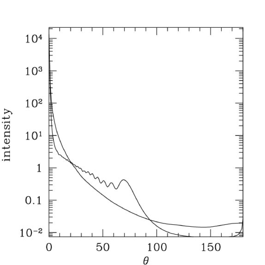
Figure 4: Unpolarized phase function for a uniform distribution of bubbles between size parameter 100 and 300 and refractive index $m=3/4$ as a function of scattering angle $\theta$. Also shown is Petzold’s phase function. The bubble phase function has peak at 70 degrees.

The main reason for the size distribution average was to remove transient spikes. This normalized phase function is scaled by $b$ calculated from Eq. 3. The volume scattering and absorption coefficients for particulates were determined from the Gordon-Morel model (Mobley, 1994; Gordon and Morel, 1983; Morel, 1988)

$$b_{p}={550\over\lambda}0.3C^{0.62}$$ (8)

$$a^{\rm Case1}(\lambda)=[a_{w}(\lambda)+0.06a_{c}^{\star}(\lambda)C^{0.65}][1+0.2\exp(-0.014(\lambda-440))]$$ (9)

Here $a_{w}(\lambda)$ is the absorption coefficient of pure water, $a_{c}^{\star}$ is the chlorophyll-specific absorption coefficient, and $C$ is the chlorophyll concentration in ${\rm mg\;m^{-3}}$ (Mobley, 1994). The chlorophyll concentration was set as constant (well-mixed) with depth and equal to 0.8${\rm mg\;m^{-3}}$ or 0.08${\rm mg\;m^{-3}}$. We used Case 1 water parameterization but assumed that not all dissolved organic material is correlated with the chlorophyll concentration. In an apparent contradiction, the wind speed which defined surface reflectance and transmittance functions due to the wind-blown water surface was set to 0. The reason for this was to estimate the effect on remote sensing properties of the sub-surface bubble clouds. However, we investigated the sensitivity of the reflectance to change in the wind speed between 0 and 10 ${\rm ms^{-1}}$, and the effect was small compared to the influence of bubbles. The azimuth direction was divided into 24 equally spaced sectors, the zenith-nadir range was divided into 20 equally spaced sectors. The profile of the bubble cloud volume fraction was determined by the expression

$$f(z)=f_{0}(f_{1}/f_{0})^{p}$$ (10)

where $f_{0}=f(z_{0})=10^{-6}$, $f_{1}=f(z_{1})=10^{-7}$, $z_{0}=0$ m, $z_{1}=8$ m, and $p=(z-z_{0})/(z_{1}-z_{0})$. Our choice of the speed of attenuation is perhaps unreasonably gradual, except for the case of stable microbubbles. On the other hand this choice is of secondary importance for the remote sensing properties of bubble clouds which are dominated by the surface volume fraction. In-water asymptotic light field is discussed by Flatau et al. (1999). The scattering was conservative. The volume attenuation was determined from the asymptotic expression (3). The probability distribution function for scattering was discretized and was set as constant throughout the depth range. We calculated the asymmetry parameter to be $g\approx 0.85$. This parameter defines the probability of photon scattering towards the forward or backward hemisphere. It is equal to 1 if all photons are scattered forward and to -1 if all photons are scattered backward.

3.2 Remote sensing reflectance

The reference model runs were performed with the 3 component system of phytoplankton, pure water, and DOM with a constant chlorophyll profile. Two cases were computed (but only one is presented), representative of clear coastal ($C=0.8$) and oceanic ($C=0.08$) water. The remote sensed reflectance is defined as

$$R_{\rm rs}(\lambda)={L_{w}(\lambda)\over E_{d}(\lambda)}$$ (11)

where $E_{d}$ is the downwelling irradiance onto the sea surface, and $L_{w}(\lambda)$ is the upwelling water-leaving radiance. The remote-sensing radiance is a measure (Mobley, 1994) of how much of the downwelling light that is incident onto the water surface is returned into the zenith direction. The remote sensing reflectances are plotted in Fig. 5. The physical importance of the remote-sensing reflectance is evident from asymptotic theories which relate $R_{\rm rs}$ to inherent optical properties (Zaneveld, 1995)

$$R_{\rm rs}\propto{\beta(\pi-\theta_{m})\over a}$$ (12)

where $\beta$ is the phase function, $\theta_{m}$ is related to the sun zenith angle, and $a$ is the absorption coefficient. Thus, $R_{\rm rs}$ is approximately proportional to the probability of back- or side-scattering, and inversly proportional to the absorption of water column. Figure 5 shows the remote-sensing reflectance for the 3- and 4-component system with and without ocean bubbles but with constant pigment amount. The total single scattering albedo is strongly influenced by scattering from air bubbles. This leads to enhanced reflectance at all wavelengths. The results for $C=0.08$ (not presented) show even larger sensitivity. In Fig 5 the gray rectangles indicate bands (wavelenghts) which are used by the current ocean color satellite instrument (SeaWiFS). It is of interest to comment on the remote sensing of pigments and bubble cloud retrievals. Consider an algorithm based on the ratio of remote-sensing reflectance and define the ratio of remote-sensing reflectances without (Chl) and with (Chl+b) microbubbles as

$${\rm ratio}(\lambda)=R_{\rm rs}^{\rm Chl}/R_{\rm rs}^{\rm Chl+b}.$$ (13)

Figure 6 shows ${\rm ratio}(\lambda)$. Performance of the pigment algorithms based on the ratio of reflectances will depend on ${\rm ratio}(\lambda_{1})/{\rm ratio}(\lambda_{2})$. Submerged microbubble clouds seem to be wavelength-selective and even the ratio algorithms may require slight systematic correction. Given the increased sensitivity of the current generation of ocean color instruments, the absolute value of the radiances at the top of the atmosphere can be used for pigment retrievals.

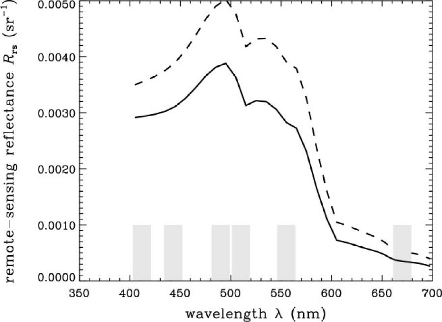
Figure 5: The solid line is the remote-sensing reflectance for the 3-component system composed of water, DOM, and particulates (no microbubbles) and the dashed line is for the 4-component system (microbubbles included). Same chlorophyll concentration (0.8${\rm mg\;m^{-3}}$) in both cases. Effective radius $r_{\rm eff}=10\mu m$. Hydrolight run with 62 layers, maximum depth 50m, maximum bubble depth 8m, 35 wavenumbers between 400-700nm, sun zenith angle 50. The grey rectangles indicate SeaWiFS (ocean color satellite) wavelengths.

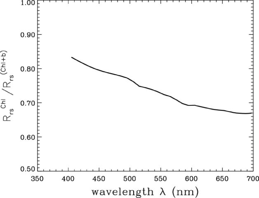
Figure 6: The ratio of remote-sensing reflectances ${\rm ratio}(\lambda)=R_{\rm rs}^{\rm Chl}/R_{\rm rs}^{\rm Chl+b}$. Same experiment as in Fig. 5.

4 Summary

Our calculations indicate that the optical effects of submerged microbubbles on the remote sensing reflectance of the ocean color are significant. These results are of importance for the retrievals of pigments from the ocean color measurements and for studies of the energetics of the ocean mixed layer. We provide information on how to reduce the systematic error due to microbubbles in pigment retrieval schemes via the ${\rm ratio}(\lambda)$. We also derive apparent optical property of bubbles - remote sensing reflectance - for the whole solar spectrum. This AOP is directly observable by the satellites and remote sensors. We expect that these and similar AOPs will have to be invoked in the case of hyperspectral retrievals for Case 2 waters where the signals from minerals, bubbles, chlorophyll, and dissolved organic material (CDOM) are not well correlated. New algorithms for current satellite instruments such as MODIS and SeaWIFS should employ this information.

We also present a global map of the volume fraction of air in water derived from daily wind speed data. We expect that such a map can be improved by knowing the day-to-day variability of the wind-wave relationship and better estimates of the volume fraction.

The paper is exploratory. Therefore, it is perhaps worth playing advocatus diaboli and speculate why the bubble clouds may not be important, at least in current satellite ocean color retrieval practice. Here are some reasons: (1) The high wind and clouds are correlated. This masks (bias) the effect of bubbles as observed from the satellites; (2) Both whitecaps (Wu, 1988b; Gordon and Wang, 1994; Frouin et al., 1996) and bubble clouds are correlated via their dependence on wind speed. Therefore, our results, as well as the hypothesis of Frouin et al. (1996), indicate that reflectance of foam has to be considered together with the reflectance due to bubble clouds. On the other hand, there are cases in which strong wind is not correlated with clouds. For example, the cross equatorial flow during the summer monsoon in the southern Indian Ocean is strong but the ITCZ position is in the northern hemisphere.

It is interesting to note that stabilized, coated microbubbles are hypothesized to be correlated to phytoplankton and CDOM concentrations; we need parameterization of this process. The optical properties of the first several meters below the surface are difficult to measure and are often removed from data due to experimental problems such as ship shadow or wave activity. This is the region where more detailed studies are needed.

References

References

- Akulichev and Bulanov (1987) Akulichev, V. and V. Bulanov, 1987: The study of sound backscattering from micro-inhomogeneities is sea water. In Progress in underwater acoustics, Merklinger, H. M., editor xv + 839. Plenum Press, New York.
- Baldy (1988) Baldy, S., 1988: Bubbles in the close vicinity of breaking waves: statistical characteristics of the generation and dispersion mechanism. J. Geophys. Res., 93(C7), 8239–8248.
- Bohren (1987) Bohren, C. F., 1987: Clouds in a glass of beer: simple experiments in atmospheric physics. Wiley, New York xv+195. The Wiley science editions.
- Bohren and Huffman (1983) Bohren, C. F. and D. R. Huffman, 1983: Absorption and scattering of light by small particles. Wiley, New York xiv + 530 p.
- Bricaud and Morel (1986) Bricaud, A. and A. Morel, 1986: Light attenuation an scattering by phytoplanktonic cells: a theoretical modeling. Appl. Opt., 25(4), 571–580.
- Bricaud et al. (1981) Bricaud, A., A. Morel, and L. Prieur, 1981: Absorption by dissolved organic matter of the sea (yellow substance) in the UV and visible domains. Limnol Oceanogr, 26, 43–53.
- Bukata (1995) Bukata, R. P., 1995: Optical properties and remote sensing of inland and coastal waters. CRC Press, Boca Raton, Fla. 362.
- Farmer and Lemon (1984) Farmer, D. M. and D. D. Lemon, 1984: The influence of bubbles on ambient noise in the ocean at high wind speeds. J. Phys. Oceanogr., 14(11), 1762–1778.
- Fiedler-Ferrari et al. (1991) Fiedler-Ferrari, N., H. M. Nussenzveig, and W. J. Wiscombe, 1991: Theory of near-critical-angle scattering from a curved interface. Phys. Rev. A, 43(2), 1005–1038.
- Flatau et al. (1999) Flatau, P. J., J. Piskozub, and J. R. V. Zaneveld, 1999: Asymptotic light field in the presence of a bubble-layer. Optics Express, 5(5), 120–124.
- Frouin et al. (1996) Frouin, R., M. Schwindling, and P.-Y. Deschamps, 1996: Spectral reflectance of sea foam in the visible and near-infrared: In situ measurements and remote sensing implications. J. Geophys. Res., 101(C6), 14361–14371.
- Gordon and Morel (1983) Gordon, H. R. and A. Y. Morel, 1983: Remote assessment of ocean color for interpretation of satellite visible imagery : a review. Springer-Verlag, New York 114. Lecture notes on coastal and estuarine studies ; 4.
- Gordon and Wang (1994) Gordon, H. R. and M. Wang, 1994: Influence of oceanic whitecaps on atmospheric correction of ocean-color sensors. Appl. Opt., 33(33), 7754–7763.
- Isao et al. (1990) Isao, K., S. Hara, K. Terauchi, and K. Kogure, 1990: Role of sub-micrometre particles in the ocean. Nature, 345(6272), 242–244.
- Johnson and Cooke (1979) Johnson, B. D. and R. C. Cooke, 1979: Bubble populations and spectra in coastal waters: a photographic approach. J. Geophys. Res., 84(C7), 3761–3766.
- Johnson and Wangersky (1987) Johnson, B. D. and P. J. Wangersky, 1987: Microbubbles: stabilization by monolayers of adsorbed particles. J. Geophys. Res., 92(C13), 14641–14647.
- Kalnay et al. (1996) Kalnay, E., M. Kanamitsu, R. Kistler, et al., 1996: The NCEP/NCAR 40-year reanalysis project. Bull. Amer. Meteorol. Soc., 77(3), 437–471.
- King et al. (1993) King, M. D., L. F. Radke, and P. V. Hobbs, 1993: Optical properties of marine stratocumulus clouds modified by ships. J. Geophys. Res., 98(D2), 2729–2739.
- Kraus and Businger (1994) Kraus, E. B. and J. A. Businger, 1994: Atmosphere-ocean interaction. Oxford University Press Clarendon Press, New York Oxford England xxii + 362 p. Oxford monographs on geology and geophysics ; no. 27.
- Medwin (1977) Medwin, H., 1977: In situ acoustic measurements of microbubbles at sea. J. Geophys. Res., 82(6), 971–976.
- Medwin and Breitz (1989) Medwin, H. and N. D. Breitz, 1989: Ambient and transient bubble spectral densities in quiescent seas and under spilling breakers. J. Geophys. Res, 94(C9), 12751–12759.
- Mobley (1994) Mobley, C. D., 1994: Light and water : radiative transfer in natural waters. Academic Press, San Diego xvii + 592.
- Mobley et al. (1994) Mobley, C. D., B. Gentili, H. R. Gordon, et al., 1994: Comparison of numerical models for computing underwater light fields. Appl. Opt., 32(36), 7484–7504.
- Morel (1988) Morel, A., 1988: Optical modeling of the upper ocean in relation to its biogenous matter content (case I waters). J. Geophys. Res., 93(C9), 10749–10768.
- Mulhearn (1981) Mulhearn, P. J., 1981: Distribution of microbubbles in coastal waters. J. Geophys. Res., 86(C7), 6429–6434.
- O’Hern et al. (1988) O’Hern, T. J., L. d’Agostino, and A. J. Acosta, 1988: Comparison of holographic and Coulter Counter measurements of cavitation nuclei in the ocean. Trans. ASME, J. Fluids Eng., 110(2), 200–207.
- Pope and Fry (1997) Pope, R. M. and E. S. Fry, 1997: Absorption spectrum (380–700nm) of pure water: II. Integrating cavity measurements. submitted to Appl. Opt.
- Stephens et al. (1990) Stephens, G. L., S.-C. Tsay, J. Stackhouse, P. W., and P. J. Flatau, 1990: The relevance of the microphysical and radiative properties of cirrus clouds to climate and climatic feedback. J. Atmos. Sci., 47(14), 1742–1753.
- Stramski (1994) Stramski, D., 1994: Gas microbubbles: An assessment of their significance to light scattering in quiescent seas. In Ocean optics XII : 13-15 June 1994, Bergen, Norway, Jaffe, J. S., editor. SPIE, Bellingham, Wash., USA 704–710. Proceedings of SPIE–the International Society for Optical Engineering ; v. 2258.
- Thorpe (1984) Thorpe, S. A., 1984: The effect of Langmuir circulation on the distribution of submerged bubbles caused by breaking wind waves. J. Fluid Mech., 14, 151–170.
- Thorpe (1995) Thorpe, S. A., 1995: Dynamical processes of transfer at the sea surface. Prog. Oceanogr., 35(4), 315–352.
- Thorpe et al. (1992) Thorpe, S. A., P. Bowyer, and D. K. Woolf, 1992: Some factors affecting the size distributions of oceanic bubbles. J. Phys. Oceanogr., 22(4), 382–389.
- Tyler (1977) Tyler, J. E., 1977: Light in the sea. Dowden, Hutchinson and Ross, Stroudsburg, Pa. New York xiii + 384 p. Benchmark papers in optics ; 3.
- Vagle and Farmer (1992) Vagle, S. and D. M. Farmer, 1992: The measurement of bubble-size distributions by acoustical backscatter. J. Atmos. Ocean. Technol., 9(5), 630–644.
- Walsh and Mulhearn (1987) Walsh, A. L. and P. J. Mulhearn, 1987: Photographic measurements of bubble populations from breaking wind waves at sea. J. Geophys. Res., 92(C13), 14553–14565.
- Wu (1988a) Wu, J., 1988a: Bubbles in the near-surface ocean: a general description. J. Geophys. Res., 93(C1), 587–590.
- Wu (1988b) Wu, J., 1988b: Variations of whitecap coverage with wind stress and water temperature. J. Phys. Oceanogr., 18(10), 1448–1453.
- Zaneveld (1995) Zaneveld, J. R. V., 1995: A theoretical derivation of the dependence of the remotely sensed reflectance of the ocean on the inherent optical properties. J. Geophys. Res., 100(C7), 13135–13142.