Abstract

By considering delta function sextupole, octupole, and decapole perturbations and using difference action-angle variable equations, we find some useful analytical formulae for the estimation of the dynamic apertures of circular accelerators due to single sextupole, single octupole, single decapole (single 2$m$ pole in general). Their combined effects are derived based on the Chirikov criterion of the onset of stochastic motions. Comparisons with numerical simulations are made, and the agreement is quite satisfactory. These formulae have been applied to determine the beam-beam limited dynamic aperture in a circular collider.

1 Introduction

One of the preoccupations of the circular accelerator designer is to estimate the influence of nonlinear forces on the single particle’s motion. These nonlinear forces manifest themselves as the systematic and random errors from optical elements, the voluntarily introduced functional ones, such as the sextupoles used for the chromaticity corrections and the octupoles used for stabilizing the particles’ collective motion, or from nonlinear beam-beam interaction forces. Even though the nonlinear forces mentioned above compared with the linear forces are usually very small, what is observed in reality, however, is that when the amplitudes of the transverse oscillation of a particle are large enough, the transverse motion might become unstable and the particle itself will finally be lost on the vacuum chamber. Apparently, the above implied maximum oscillation amplitudes, $A_{x,y}$, corresponding to the stable motions are functions of the specific longitudinal position, $s$, along the machine, and these functions $A_{x,y}(s)$ are the so-called dynamic apertures of the machine. A reasonably designed machine should satisfy the condition $A_{x,y}(s)\geq M_{x,y}(s)$, where $M_{x,y}(s)$ are the mechanical cross-section dimensions of the vacuum chamber.

Needless to say the dynamic aperture problem in circular accelerators is one of the most challenging research topics for accelerator physicists, and the relevant methods adopted to treat this problem are quite different analytically and numerically. In this paper we will show how single sextupole, single octupole, and single decapole (single 2$m$ pole in general) in the machine

limit the dynamic aperture and what is their combined effect if there are more than one nonlinear element. From the established analytical formulae for the dynamic aperture one gets the scaling laws which relate the nonlinear perturbation strengths, beta functions, and the dynamic apertures. To test the validity of these formulae, comparisons with some numerical simulation have been made. As an interesting application the beam-beam limited dynamic apertures in a circular collider have been discussed.

2 Hamiltonian Formalism

The Hamiltonian formulation of dynamics is best known not only for its deep physical and philosophical inspiration to the physicists, but also for its technical convenience in solving various nonlinear dynamical problems. The general Hamiltonian for a particle of rest mass, $m_{0}$, and charge, $e$, in a magnetic vector potential, $\bf A$, and electric potential, $\Phi$, is expressed as:

$${\cal H}(q,p,t)=e\Phi+c\left(({\bf p}-e{\bf A})^{2}+m_{0}c^{2}\right)^{1/2}$$ (1)

where $c$ is the velocity of light and $\bf p$ is the momentum with its components, $p_{i}$, conjugate to the space coordinates, $q_{i}$. The equations of motion can be readily written in terms of Hamilton’s equations:

$${dp_{i}\over dt}=-{\partial{\cal H}\over\partial q_{i}}$$ (2)

$${dq_{i}\over dt}={\partial{\cal H}\over\partial p_{i}}$$ (3)

For our specific dynamic problems in a circular accelerator it is convenient to chose curvilinear coordinates instead of Cartesian ones for us to describe the trajectory of a particle near an a priori known closed orbit. The Hamiltonian in the new system, $(x,s,y)$ (where $x,s$, and $y$ denote the coordinates in the Frenet-Serret normal, tangent, and binormal triorthogonal and right-handed coordinate system), is given by [1]^-[7]:

$$H_{t}(q,p,t)=e\Phi+c\left((p_{x}-eA_{x})^{2}+(p_{y}-eA_{y})^{2}+\left({p_{s}-eA_{s}\over 1+x/\rho}\right)^{2}+m_{0}c^{2}\right)^{1/2}$$ (4)

where $\rho$ is the radius of curvature and the torsion of the closed orbit is everywhere zero. Since it is useful to use the variable, $s$, as the independent variable rather than time, $t$, one gets the new Hamiltonian by using a simple canonical transformation:

$$H_{s}=-eA_{s}-(1+x/\rho)\left({1\over c^{2}}(E^{2}-m_{0}^{2}c^{4})-(p_{x}-eA_{x})^{2}-(p_{y}-eA_{y})^{2}\right)^{1/2}-e\Phi$$ (5)

Noting that the term ${1\over c^{2}}(E^{2}-m_{0}^{2}c^{4})$ in eq. 5 is equal to $P^{2}$ with $P$ being the total mechanical momentum of the particle, by using another trivial canonical transformation:

$${\bar{q}}=q,{\bar{s}}=s,{\bar{p}}_{x,y}={p_{x,y}\over P_{0}},H={H_{s}\over P_{0}}$$ (6)

one gets another Hamiltonian:

$$H=-{eA_{s}\over P_{0}}-(1+x/\rho)\left({P\over P_{0}}-({\bar{p}}_{x}-{eA_{x}\over P_{0}})^{2}-({\bar{p}}_{y}-{eA_{y}\over P_{0}})^{2}\right)^{1/2}-{e\Phi\over P_{0}}$$ (7)

where $P_{0}$ is the mechanical momentum of the reference particle, and $P=P_{0}+\Delta P$. Inserting $eA_{s}/P_{0}$ in eq. 7 by:

$${eA_{s}\over P_{0}}=-{B_{y}x^{2}\over 2\rho^{2}B_{0}}-{1\over B_{0}\rho}\sum_{n=1}^{\infty}{1\over n!}{\partial^{n-1}B_{y}\over\partial x^{n-1}}|_{x=0,y=0}(x+iy)^{n}$$ (8)

one gets finally the Hamiltonian which serves as the starting point of most of the dynamical problems concerning circular accelerators:

$$H={x^{2}B_{y}|_{x=0,y=0}\over 2\rho^{2}B_{0}}+{1\over B_{0}\rho}\sum_{n=1}^{\infty}{1\over n!}{\partial^{n-1}B_{y}\over\partial x^{n-1}}|_{x=0,y=0}(x+iy)^{n}$$

$$-(1+x/\rho)\left(1+{\Delta P\over P_{0}}-\left({\bar{p}}_{x}-{eA_{x}\over P_{0}}\right)^{2}-\left({\bar{p}}_{y}-{eA_{y}\over P_{0}}\right)^{2}\right)^{1/2}-{e\Phi\over P_{0}}$$ (9)

where $B_{0}$ is the bending magnetic field on the orbit of the reference particle, and $B_{y}$ in general is a complex variable.

3 Analytical formulae for dynamic apertures

To start with we consider the linear horizontal motion of the reference particle (no energy deviation) in the horizontal plane (y=0) assuming that the magnetic field is only transverse ($A_{x}=A_{y}=0$) and has no skew fields, and $\Phi$ is a constant. The Hamiltonian can be simplified as

$$H={p^{2}\over 2}+{K(s)\over 2}x^{2}$$ (10)

where $x$ denotes normal plane coordinate, $p=dx/ds$, and $K(s)$ is a periodic function satisfying the relation

$$K(s)=K(s+L)$$ (11)

where $L$ is the circumference of the ring. The solution of the deviation, $x$, is found to be

$$x=\sqrt{\epsilon_{x}\beta_{x}(s)}\cos(\phi(s)+\phi_{0})$$ (12)

where

$$\phi(s)=\int_{0}^{s}{ds\over\beta_{x}(s)}$$ (13)

As an essential step towards further discussion on the motions under nonlinear perturbation forces, we introduce action-angle variables and the Hamiltonian expressed in these new variables:

$$\Psi=\int_{0}^{s}{ds^{\prime}\over\beta_{x}(s^{\prime})}+\phi_{0}$$ (14)

$$J={\epsilon_{x}\over 2}={1\over 2\beta_{x}(s)}\left(x^{2}+\left(\beta_{x}(s)x^{\prime}-{\beta_{x}^{\prime}x\over 2}\right)^{2}\right)$$ (15)

$$H(J,\Psi)={J\over\beta_{x}(s)}$$ (16)

Since $H(J,\Psi)=J/\beta_{x}(s)$ is still a function of the independent variable, $s$, we will make another canonical transformation to freeze the new Hamiltonian:

$$\Psi_{1}=\Psi+{2\pi\nu\over L}-\int_{0}^{s}{ds^{\prime}\over\beta_{x}(s^{\prime})}$$ (17)

$$J_{1}=J$$ (18)

$$H_{1}={2\pi\nu\over L}J_{1}$$ (19)

Before going on further, let’s remember the relation between the last action-angle variables and the particle deviation $x$:

$$x=\sqrt{2J_{1}\beta_{x}(s)}\cos\left(\Psi_{1}-{2\pi\nu\over L}s+\int_{0}^{s}{ds^{\prime}\over\beta_{x}(s^{\prime})}\right)$$ (20)

Being well prepared, we start our journey to find out the limitations of the nonlinear forces on the stability of the particle’s motion. To facilitate the analytical treatment of this complicated problem we consider at this stage only sextupoles and octupoles (no skew terms) and assume that the contributions from the sextupoles and octupoles in a ring can be made equivalent to a point sextupole and a point octupole. The perturbed one dimensional Hamiltonian can thus be expressed:

$$H={p^{2}\over 2}+{K(s)\over 2}x^{2}+{1\over 3!B\rho}{\partial^{2}B_{z}\over\partial x^{2}}x^{3}L\sum_{k=-\infty}^{\infty}\delta(s-kL)+{1\over 4!B\rho}{\partial^{3}B_{z}\over\partial x^{3}}x^{4}L\sum_{k=-\infty}^{\infty}\delta(s-kL)$$ (21)

Representing eq. 21 by action-angle variables ($J_{1}$ and $\Psi_{1}$), and using

$$B_{z}=B_{0}(1+xb_{1}+x^{2}b_{2}+x^{3}b_{3})$$ (22)

one has

$$H={2\pi\nu\over L}J_{1}+{(2J_{1}\beta_{x}(s_{1}))^{3/2}\over 3\rho}b_{2}L\cos^{3}\Psi_{1}\sum_{k=-\infty}^{\infty}\delta(s-kL)$$

$$+{(J_{1}\beta_{x}(s_{2}))^{2}\over\rho}b_{3}L\cos^{4}\Psi_{1}\sum_{k=-\infty}^{\infty}\delta(s-kL)$$ (23)

where $s_{1}$ and $s_{2}$ are just used to differentiate the locations of the sextupole and the octupole perturbations. By virtue of Hamiltonian one gets the differential equations for $\Psi_{1}$ and $J_{1}$

$${dJ_{1}\over ds}=-{\partial H_{1}\over\partial\Psi_{1}}$$ (24)

$${d\Psi_{1}\over ds}={\partial H_{1}\over\partial J_{1}}$$ (25)

$${dJ_{1}\over ds}=-{(2J_{1}\beta_{x}(s_{1}))^{3/2}\over 3\rho}b_{2}L{d\cos^{3}\Psi_{1}\over d\Psi_{1}}\sum_{k=-\infty}^{\infty}\delta(s-kL)$$

$$-{(J_{1}\beta_{x}(s_{2}))^{2}\over\rho}b_{3}L{d\cos^{4}\Psi_{1}\over d\Psi_{1}}\sum_{k=-\infty}^{\infty}\delta(s-kL)$$ (26)

$${d\Psi_{1}\over ds}={2\pi\nu\over L}+{\sqrt{2}J_{1}^{1/2}\beta_{x}(s_{1})^{3/2}\over\rho}b_{2}L\cos^{3}\Psi_{1}\sum_{k=-\infty}^{\infty}\delta(s-kL)$$

$$+{2\beta_{x}^{2}(s_{2})\over\rho}J_{1}b_{3}L\cos^{4}\Psi_{1}\sum_{k=-\infty}^{\infty}\delta(s-kL)$$ (27)

We now change these differential equations to the difference equations which are suitable to analyse the possibilities of the onset of stochasticity [8][9]. Since the perturbations have a natural periodicity of $L$ we will sample the dynamic quantities at a sequence of $s_{i}$ with constant interval $L$ assuming that the characteristic time between two consecutive adiabatic invariance breakdown intervals is shorter than $L/c$. The differential equations in eqs. 26 and 27 are reduced to

$$\overline{J_{1}}=\overline{J_{1}}(\Psi_{1},J_{1})$$ (28)

$$\overline{\Psi_{1}}=\overline{\Psi_{1}}(\Psi_{1},J_{1})$$ (29)

where the bar stands for the next sampled value after the corresponding unbarred previous value.

$$\overline{J_{1}}=J_{1}-{(2J_{1}\beta_{x}(s_{1}))^{3/2}\over 3\rho}b_{2}L{d\cos^{3}\Psi_{1}\over d\Psi_{1}}-{(J_{1}\beta_{x}(s_{2}))^{2}\over\rho}b_{3}L{d\cos^{4}\Psi_{1}\over d\Psi_{1}}$$ (30)

$$\overline{\Psi_{1}}=\Psi_{1}+{2\pi\nu}+{\sqrt{2}\beta_{x}(s_{1})^{3/2}\overline{J_{1}}^{1/2}\over\rho}b_{2}L\cos^{3}\Psi_{1}+{2\beta_{x}(s_{2})^{2}\over\rho}\overline{J_{1}}b_{3}L\cos^{4}\Psi_{1}$$ (31)

Eqs. 30 and 31 are the basic difference equations to study the nonlinear resonance and the onset of stochasticities considering sextupole and octupole perturbations. By using trigonometric relation

$$\cos^{m}\theta\cos n\theta=2^{-m}\sum_{r=0}^{m}{m!\over(m-r)!r!}\cos(n-m+2r)\theta$$ (32)

one has

$$\cos^{3}\theta={2\over 2^{3}}(\cos 3\theta+3\cos\theta)$$ (33)

$$\cos^{4}\theta={1\over 2^{4}}(2\cos 4\theta+8\cos 2\theta+{4!\over((4/2)!)^{2}})$$ (34)

If the tune $\nu$ is far from the resonance lines $\nu=m/n$, where $m$ and $n$ are integers, the invariant tori of the unperturbed motion are preserved under the presence of the small perturbations by virtue of the Kolmogorov-Arnold-Moser (KAM) theorem. If, however, $\nu$ is close to the above mentioned resonance line, under some conditions the KAM invariant tori can be broken.

Consider first the case where there is only one sextupole located at $s=s_{1}$ with $\beta_{x}(s_{1})$. Taking the third order resonance, $m/3$, for example, we keep only the sinusoidal function with phase $3\Psi_{1}$ in eq. 30 and the dominant phase independent nonlinear term in eq. 31, and as the result, eqs. 30 and 31 become

$$\overline{J_{1}}=J_{1}+A\sin 3\Psi_{1}$$ (35)

$$\overline{\Psi_{1}}=\Psi_{1}+B\overline{J_{1}}$$ (36)

with

$$A={(2J_{1}\beta_{x}(s_{1}))^{3/2}\over 4}\left({b_{2}L\over\rho}\right)$$ (37)

$$B=\sqrt{2}\beta_{x}(s_{1})^{3/2}J_{1}^{-1/2}\left({b_{2}L\over\rho}\right)$$ (38)

where we have dropped the constant phase in eq. 31 and take the maximum value of $\cos^{3}({\Psi_{1}})$, 1. It is helpful to transform eqs. 37 and 38 into the form so-called standard mapping [9] expressed as

$$\overline{I}=I+K_{0}\sin\theta$$ (39)

$$\overline{\theta}=\theta+\overline{I}$$ (40)

with $\theta=3\Psi$, $I=3BJ_{1}$ and $K_{0}=3AB$. By virtue of the Chirikov criterion [9] it is known that when $|K_{0}|\geq 0.97164$ [10] resonance overlapping occurs which results in particles’ stochastic motions and diffusion processes. Therefore,

$$|K_{0}|\ \leq 1$$ (41)

can be taken as a natural criterion for the determination of the dynamic aperture of the machine. Putting eqs. 37 and 38 into eq. 41, one gets

$$|K_{0}|=3J_{1}\beta_{x}(s_{1})^{3}\left({|b_{2}|L\over\rho}\right)^{2}\leq 1$$ (42)

and consequently, one finds maximum $J_{1}$ corresponding to a $m/3$ resonance

$$J_{1}\leq J_{max,sext}={1\over 3\beta_{x}(s_{1})^{3}}\left({\rho\over|b_{2}|L}\right)^{2}$$ (43)

The dynamic aperture of the machine is therefore

$$A_{dyna,sext}=\sqrt{2J_{max,sext}\beta_{x}(s)}={\sqrt{2\beta_{x}(s)}\over\sqrt{3}\beta_{x}(s_{1})^{3/2}}\left({\rho\over|b_{2}|L}\right)$$ (44)

Eq. 44 gives the dynamic aperture of a sextuple strength determined case. The reader can confirm that if we keep $\sin(\Psi_{1})$ term instead of $\sin(3\Psi_{1})$ in eq. 35, one arrives at the same expression for $A_{dyna,sext}$ as expressed in eq. 44.

Secondly, we consider the case of single octupole located at $s=s_{2}$ with $\beta_{x}(s_{2})$. Taking the forth order resonance, $m/4$, for example, we keep only the sinusoidal function with phase $4\Psi_{1}$ in eq. 30 and the dominant phase independent nonlinear term in eq. 31, and as the result, we have eqs. 30 and 31 reduced to

$$\overline{J_{1}}=J_{1}+A\sin 4\Psi_{1}$$ (45)

$$\overline{\Psi_{1}}=\Psi_{1}+B\overline{J_{1}}$$ (46)

with

$$A={(J_{1}\beta_{x}(s_{2}))^{2}\over 2}\left({b_{3}L\over\rho}\right)$$ (47)

$$B={2\beta_{x}(s_{2})^{2}}\left({b_{3}L\over\rho}\right)$$ (48)

where we have dropped the constant phase in eq. 31 and take the maximum value of $\cos^{4}({\Psi_{1}})$, 1. By using Chirikov criterion, one gets

$$J_{1}\leq J_{max,oct}={1\over 2\beta_{x}(s_{2})^{2}}\left({\rho\over|b_{3}|L}\right)$$ (49)

and the corresponding dynamic aperture:

$$A_{dyna,oct}=\sqrt{2J_{max,oct}\beta_{x}(s)}={\sqrt{\beta_{x}(s)}\over\beta_{x}(s_{2})}\sqrt{\rho\over|b_{3}|L}$$ (50)

Thirdly, without repeating, we give directly the dynamic aperture due to a decapole located at $s=s_{3}$:

$$A_{dyna,deca}=\sqrt{2\beta_{x}(s)}\left({1\over 5\beta_{x}^{5}(s_{3})}\right)^{1/6}\left({\rho\over|b_{4}|L}\right)^{1/3}$$ (51)

where $b_{4}$ is the coefficient of the decapole strength. Finally, we give the general expression of the dynamic aperture in the horizontal plane ($z=0$) of a single $2m$ ($m\geq 3$) pole component:

$$A_{dyna,2m}=\sqrt{2\beta_{x}(s)}\left({1\over m\beta_{x}^{m}(s(2m))}\right)^{1\over 2(m-2)}\left({\rho\over|b_{m-1}|L}\right)^{1/(m-2)}$$ (52)

where $s(2m)$ is the location of this multipole. Eq. 52 gives us useful scaling laws, such as $A_{dyna,2m}\propto\left({\rho\over|b_{m-1}|L}\right)^{1/(m-2)}$, and $A_{dyna,2m}\propto\left({1\over\beta_{x}^{m}(s(2m))}\right)^{1\over 2(m-2)}$.

If there is more than one nonlinear component, how can one estimate their collective effect ? Fortunately, one can distinguish two cases:

• If the components are independent, i.e. there are no special phase and amplitude relations between them, the total dynamic aperture can be calculated as:

$$A_{dyna,total}={1\over\sqrt{\sum_{i}{1\over A_{dyna,sext,i}^{2}}+\sum_{j}{1\over A_{dyna,oct,j}^{2}}+\sum_{k}{1\over A_{dyna,deca,k}^{2}}+\cdot\cdot\cdot}}$$ (53)

• If the nonlinear components are dependent, i.e. there are special phase and amplitude relations between them (for example, in reality, one use some additional sextupoles to cancel the nonlinear effects of the sextupoles used to make chromaticity corrections), there is no general formula as eq. 53 to apply.

In the above discussion we have restricted us to the case where particles are moving in the horizontal plane, and the one dimensional dynamic aperture formulae expressed in eqs. 44, 50, 51 and 53, are the maximum stable horizontal excursion ranges with the vertical displacement $y=0$. In the following we will show briefly how to estimate the dynamic aperture in 2 dimensions when there is coupling between the horizontal and vertical planes. Now we consider the case where only one sextupole is located at $s=s_{1}$, and we have the corresponding Hamiltonian expressed as follows:

$$H={p_{x}^{2}\over 2}+{K_{x}(s)\over 2}x^{2}+{p_{y}^{2}\over 2}+{K_{y}(s)\over 2}y^{2}+{1\over 3!B\rho}{\partial^{2}B_{z}\over\partial x^{2}}(x^{3}-3xy^{2})L\sum_{k=-\infty}^{\infty}\delta(s-kL)$$ (54)

Generally speaking, there exists no universal criterion to determine the start up of stochastic motions in 2D. Fortunately, in our specific case, we find out the similarity between the Hamiltonian expressed in eq. 54 and that of the Hénon and Heiles problem which has been much studied in literature [11]. The Hénon and Heiles problem’s Hamiltonian is given by

$$H_{H\&H}={1\over 2}\left(x^{2}+p_{x}^{2}+y^{2}+p_{y}^{2}+2y^{2}x-{2\over 3}x^{3}\right)$$ (55)

when $H_{H\&H}>1/6$ the motion becomes unstable. The intuition we get from this conclusion is that there should exist a similar criterion for our problem, i.e. to have stable 2D motion one should have $H\leq H_{max}$. Note that $K_{x}(s)$ and $K_{y}(s)$ in eq. 54 are equal to unity in the Hénon and Heiles problem’s Hamiltonian. The previous one dimensional result helps us now to find $H_{max}$. When $y=0$ one has $H_{max}\propto A^{2}_{dyna,sext,x}$, since $x\leq A_{dyna,sext,x}$. When $y\neq 0$, the crossing terms in eqs. 54 and 55 will play the role of exchanging energy between the two planes, and for a given set of $x$ and $y$ the total energy of the coupled system can not exceed $H_{max}$. If we define $A_{dyna,sext,y}$ is the dynamic aperture in $y$-plane, one has:

$$\beta_{x}(s_{1})A_{dyna,sext,x}^{2}=\beta_{y}(s_{1})A^{2}_{dyna,sext,y}+\beta_{x}(s_{1})x^{2}$$ (56)

or:

$$A_{dyna,sext,y}=\sqrt{{\beta_{x}(s_{1})\over\beta_{y}(s_{1})}(A^{2}_{dyna,sext,x}-x^{2})}$$ (57)

where $\beta_{y}(s_{1})$ is the vertical beta function where the sextupole is located and $A_{dyna,sext,x}$ is given by eq. 44. Different from eq. 52, the derivation of eq. 57 is quite intuitive, hinted by the Hénon and Heiles problem which has been studied numerically instead of analytically in literature. From eq. 57 one understands that the difference between $A_{dyna,sext,y}$ and $A_{dyna,sext,x}$ comes from $\sqrt{\beta_{x}(s_{1})/\beta_{y}(s_{1})}$. If there are many sextupoles in a ring one usually has $A_{dyna,sext,x}\approx A_{dyna,sext,y}$ since $\beta_{x}(s_{i})$ will not be always larger or smaller than $\beta_{y}(s_{i})$.

4 Comparison with simulation results

To verify the validity of eqs. 44, 50, 53, and 57, we compare the dynamic apertures of some special cases by using these analytical formulae with a computer code called BETA [12]. Taking the lattice of Super-ACO as an example, we show the schematic layout of the machine in Fig. 1.

Figure 1: The schematic layout of Super-ACO.

The horizontal beta function distribution and the working point in the third order tune diagram are given in Figs. 2 and 3, respectively. From Fig. 2 one finds that the horizontal beta function at the beginning and the end of the one turn mapping is 5.6 m. In the following numerical simulations the dynamic apertures correspond to $\beta_{x}(s)=\beta_{x}(0)=5.6$ m and it will also be used in the analytical formulae. Defining the sextupole, octupole, and decapole strengths $S=b_{2}L/\rho$ (1/m²), $O=b_{3}L/\rho$ (1/m³), $D=b_{4}L/\rho$ (1/m${}^{4})$, respectively, we make now a rather systematic comparison.

• A sextupole is located at $s=s_{1}$ with $S(s_{1})=1$ and $\beta_{x}(s_{1})=13.6$ m, and its influence on the horizontal dynamic aperture is illustrated in Figs. 4 and 5. From eq. 44 one gets analytically that $A_{dyna,sext}=0.0385$ m compared with the numerical value of 0.04 m.

• An octupole is located at $s=s_{1}$ with $O(s_{1})=10$ and $\beta_{x}(s_{1})=13.6$ m, and its influence on the horizontal dynamic aperture is illustrated in Figs. 6 and 7. From eq. 50 one gets analytically that $A_{dyna,oct}=0.055$ m compared with the numerical value of 0.054 m.

• The validity of eq. 51 has been checked also. If a decapole with strength $D=1000$ is located at $s=s_{1}$, the dynamic aperture in horizontal plane is shown in Figs. 8 and 9. From eq. 51 one gets $A_{dyna,deca}=0.022$ m compared with the numerical value of 0.024 m.

• A sextupole of $S=2$ and a octupole of $O=62$ are located at $s=s_{1}$ and $\beta_{x}(s_{1})=13.6$ m, and their combined influence on the horizontal dynamic aperture is shown in Figs. 10 and 11. From eq. 53 one gets $A_{dyna,total}=0.0145$ m compared with the numerical value of 0.016 m.

  
  
  

  Figure 2: The horizontal beta function distribution of Super-ACO ($\beta_{x}(0)=5.6$ m).

  
  

  Figure 3: The tune diagram of the third order of Super-ACO, where the cross indicates the working point of the machine.

  
  
  

  Figure 4: The dynamic aperture plot ($S(s_{1})=1$ and $\beta_{x}(s_{1})=13.6$ m).

  

  Figure 5: The horizontal phase space ($S(s_{1})=1$ and $\beta_{x}(s_{1})=13.6$ m).

  
  

  Figure 6: The dynamic aperture plot ($O(s_{1})=10$ and $\beta_{x}(s_{1})=13.6$ m).

  
  

  Figure 7: The horizontal phase space ($O(s_{1})=10$ and $\beta_{x}(s_{1})=13.6$ m).

  
  

  Figure 8: The dynamic aperture plot ($D(s_{1})=1000$ and $\beta_{x}(s_{1})=13.6$ m).

  
  

  Figure 9: The horizontal phase space ($D(s_{1})=1000$ and $\beta_{x}(s_{1})=13.6$ m).

  
  

  Figure 10: The dynamic aperture plot ($S(s_{1})=2$, $O(s_{1})=62$, and $\beta_{x}(s_{1})=13.6$ m).

  

  Figure 11: The horizontal phase space ($S(s_{1})=2$, $O(s_{1})=62$, and $\beta_{x}(s_{1})=13.6$ m).

• A sextupole of $S=2$ and a octupole of $O=62$ are located at $s=s_{1}$, $\beta_{x}(s_{1})=13.6$ m, and $s=s_{2}$, $\beta_{x}(s_{2})=15.18$ m, respectively, and their combined influence on the horizontal dynamic aperture is shown in Figs. 12 and 13. From eq. 53 one gets $A_{dyna,total}=0.0138$ m compared with the numerical value of 0.0135 m.

• Four sextupoles of $S=2$ are located at $s=s_{1,2,3,4}$ with $\beta_{x}(s_{1})=13.6$ m, $\beta_{x}(s_{2})=15.18$ m, $\beta_{x}(s_{3})=7.8$ m, and $\beta_{x}(s_{4})=6.8$ m, respectively, and their combined influence on the horizontal dynamic aperture is given in Figs. 14 and 15. From eq. 53 one obtained the analytical value $A_{dyna,total}=0.012$ m.

• We show how the dynamic apertures depend on the strengths of sextupole and octupole. Fig. 16 shows the comparison between the analytical (solid line) and the numerical (dotted) results for a sextupole located at $s=s_{1}$ in the machine shown in Fig. 2. Obviously, $A_{dyna,sext}$ scales with $1/S$. Fig. 17 gives the similar comparison for an octupole located at $s=s_{2}$, and confirms that $A_{dyna,oct}$ scales with $1/\sqrt{S}$.

• Now we change the tune of the machine a little bit (from $\nu_{x}=1.7$ to $\nu_{x}=1.565$), and the corresponding horizontal beta function distribution and the third order tune diagram are shown in Figs. 18 and 19. It is known that in this case $\beta_{x}(0)=5.1$ m. A sextupole of $S=2$ is located a $s=s_{1}$ with $\beta_{x}(s_{1})=12.42$ m, and its influence on the dynamic aperture is shown in Figs. 20 and 21. From eq. 44 one finds $A_{dyna,sext}=0.021$ m compared with the numerical value of 0.02 m.

• Finally, a 2D dynamic aperture is calculated numerically and analytically. If a sextupole of $S=2$ is located at $s_{2}$ in the same lattice as in case (1) with $\beta_{x}=15.18$ m and $\beta_{y}=4.26$ m, the 2D dynamic aperture is calculated by using BETA and eq. 57 as shown in Fig. 22 and Fig. 23, respectively. The peak analytical dynamic apertures in horizontal and vertical planes are 0.0163 m and 0.031 m, compared with the numerical results of 0.017 m and 0.034 m, respectively.

Figure 12: The dynamic aperture plot ($S(s_{1})=2$, $O(s_{2})=62$, $\beta_{x}(s_{1})=13.6$ m, and $\beta_{x}(s_{2})=15.18$ m ).

Figure 13: The horizontal phase space ($S(s_{1})=2$, $O(s_{2})=62$, $\beta_{x}(s_{1})=13.6$ m, and $\beta_{x}(s_{2})=15.18$ m).

Figure 14: The dynamic aperture plot ($S(s_{1,2,3,4})=2$, $\beta_{x}(s_{1})=13.6$ m, $\beta_{x}(s_{2})=15.18$ m, $\beta_{x}(s_{3})=7.8$ m, and $\beta_{x}(s_{4})=6.8$ m).

Figure 15: The horizontal phase space ($S(s_{1,2,3,4})=2$, $\beta_{x}(s_{1})=13.6$ m, $\beta_{x}(s_{2})=15.18$ m, $\beta_{x}(s_{3})=7.8$ m, and $\beta_{x}(s_{4})=6.8$ m).

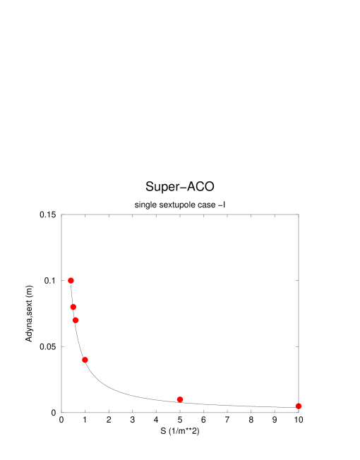
Figure 16: The dynamic aperture of Super-ACO vs S ($S=b_{2}L/\rho$) at $s_{1}$.

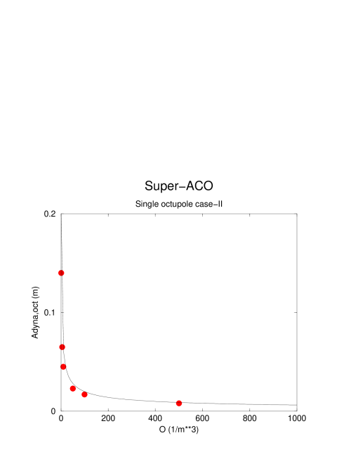
Figure 17: The dynamic aperture of Super-ACO vs O ($O=b_{3}L/\rho$) at $s_{2}$.

Figure 18: The horizontal beta function distribution of modified Super-ACO ($\beta_{x}(0)=5.1$ m).

Figure 19: The tune diagram of the third order of modified Super-ACO, where the cross indicates the working point of the machine.

Figure 20: The dynamic aperture plot ($S(s_{1})=2$ and $\beta_{x}(s_{1})=12.42$ m).

Figure 21: The horizontal phase space ($S(s_{1})=2$ and $\beta_{x}(s_{1})=12.42$ m).

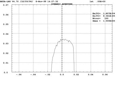
Figure 22: The 2D dynamic aperture of Super-ACO with S=2 located at $s_{2}$ with $\beta_{x}(s_{2})=15.18$ m and $\beta_{y}(s_{2})=4.26$ m.

Figure 23: The analytical estimation of the 2D dynamic aperture of Super-ACO with S=2 located at $s_{2}$ with $\beta_{x}(s_{2})=15.18$ m and $\beta_{y}(s_{2})=4.26$ m.

To make the comparison much more clear we illustrate the machine parameters in Table 1 and the comparison results in Table 2.

The agreement between the analytical and the numerical simulation results is quite good. The fact that the analytically estimated 2D dynamic aperture agrees well with that calculated by the numerical method shows that the method we have used to treat the two coupled nonlinear oscillators is a reasonable heuristic procedure.

Case	Multipole strength	beta function (m)
1	$S(s_{1})=2$ (1/m2)	$\beta_{x}(s_{1})=13.6$
2	$O(s_{1})=10$ (1/m3)	$\beta_{x}(s_{1})=13.6$
3	$D(s_{1})=1000$ (1/m4)	$\beta_{x}(s_{1})=13.6$
4	$S(s_{1})=2$ (1/m2), $O(s_{1})=62$ (1/m3)	$\beta_{x}(s_{1})=13.6$
5	$S(s_{1})=2$ (1/m2), $O(s_{2})=62$ (1/m3)	$\beta_{x}(s_{1})=13.6$ , $\beta(s_{2})=15.18$
6	$S(s_{1,2,3,4})=2$ (1/m2)	$\beta_{x}(s_{1,2,3,4})=$13.6, 15.18, 7.8, 6.8
8	$S(s_{1})=2$ (1/m2)	$\beta_{x}(s_{1})=12.42$ , $\beta_{x}(0)=5.1$
9	$S(s_{1})=2$ (1/m2)	$\beta_{x}(s_{2})=15.18$

Table 1: summary of parameters

Case	$A_{dyna,analy.}$ (m)	$A_{dyna,numer.}$ (m)
1	$0.0385$	$0.04$
2	0.055	$0.054$
3	$0.022$	$0.024$
4	$0.0145$	$0.016$
5	$0.0138$	$0.0135$
6	$0.012$	$0.0135$
8	$0.021$	$0.02$
9	$A_{x}=0.0163$ , $A_{y}=0.031$	$A_{x}=0.017$, $A_{y}=0.034$

Table 2: summary of comparison results

5 Beam-beam interaction limited dynamic apertures

Since we are interested in the single particle motion under beam-beam forces, the incoherent force should be taken into account [13]:

$$F_{r,in}(r)=\pm{nq^{2}(1+\beta^{2})\over 2\pi\epsilon_{0}r}\left(1-\exp\left(-{r^{2}\over 2\sigma^{2}}\right)\right)$$ (58)

where $n$ is the line particle number density, $\beta$ is the particle’s velocity in units of the speed of light, $q$ is the particle’s electric charge, $\epsilon_{0}$ is the permitivity in vacuum, $r$ is the transverse offset of a particle with respect to the center of the counter-rotating colliding bunch, $\sigma$ is the standard deviation of the Gaussian transverse charge density distribution, the positive and the negative signs correspond to the colliding bunches with the same or opposite charges, respectively. Now we expand $F_{r,in}(r)$ into Taylor series:

$$F_{r,in}(r)=\pm{nq^{2}\over\pi\epsilon_{0}}\left({1\over 2\sigma^{2}}r-{1\over 8\sigma^{4}}r^{3}+{1\over 48\sigma^{6}}r^{5}-{1\over 384\sigma^{8}}r^{7}+\cdot\cdot\cdot\right)$$ (59)

where we take $\beta=1$. To start with, we consider the particle’s motion in horizontal plane ($y=0$) and consider only the delta function nonlinear beam-beam forces coming from one IP. The differential equation of motion can be expressed as:

$${d^{2}x\over ds^{2}}+K_{x}(s)x=\pm{nq^{2}\over\pi\epsilon_{0}m_{0}c^{2}\gamma}({1\over 2\sigma^{2}}x-{1\over 8\sigma^{4}}x^{3}+{1\over 48\sigma^{6}}x^{5}$$

$$-{1\over 384\sigma^{8}}x^{7}+\cdot\cdot\cdot)L\sum_{k=-\infty}^{\infty}\delta(s-kL)$$ (60)

where $K_{x}(s)$ describes the linear focusing of the lattice in the horizontal plane, $m_{0}c^{2}$ is the rest energy of the particle, $\gamma$ is the normalized particle’s energy, and $L$ is the circumference of the circular collider. The corresponding Hamiltonian is expressed as:

$$H={p_{x}^{2}\over 2}+{K_{x}(s)\over 2}x^{2}\mp{nq^{2}\over\pi\epsilon_{0}m_{0}c^{2}\gamma}({1\over 4\sigma^{2}}x^{2}-{1\over 32\sigma^{4}}x^{4}+{1\over 288\sigma^{6}}x^{6}$$

$$-{1\over 3072\sigma^{8}}x^{8}+\cdot\cdot\cdot)L\sum_{k=-\infty}^{\infty}\delta(s-kL)$$ (61)

where $p_{x}=dx/ds$.

To make use of the general dynamic aperture formulae shown in section 3, one needs only to find the equivalence relations by comparing two Hamiltonians expressed in eqs. 21 and 61, respectively, and it is found that:

$${b_{3}\over\rho}L={N_{e}q^{2}\over 8\pi\epsilon_{0}m_{0}c^{2}\gamma\sigma^{4}}$$ (62)

$${b_{5}\over\rho}L={N_{e}q^{2}\over 48\pi\epsilon_{0}m_{0}c^{2}\gamma\sigma^{6}}$$ (63)

$${b_{7}\over\rho}L={N_{e}q^{2}\over 384\pi\epsilon_{0}m_{0}c^{2}\gamma\sigma^{8}}$$ (64)

and so on, where we have replaced $nL$ by $N_{e}$ which is the particle population inside a bunch. Till now one can calculate all kinds of dynamic apertures due to nonlinear beam-beam forces. For example, one can get the dynamic apertures due to the beam-beam octupole nonlinear force:

$$A_{dyna,8,x}={\sqrt{\beta_{x}(s)}\over\beta_{x}(s^{*})}\sqrt{\rho\over|b_{3}|L}$$

$$={\sqrt{\beta_{x}(s)}\over\beta_{x}(s^{*})}\left({8\pi\epsilon_{0}m_{0}c^{2}\gamma\sigma^{4}\over N_{e}q^{2}}\right)^{1/2}$$ (65)

and

$$A_{dyna,8,y}=\sqrt{{\beta_{x}(s^{*})\over\beta_{y}(s^{*})}(A^{2}_{dyna,8,x}-x^{2})}$$ (66)

where $s^{*}$ is the IP position. If we measure dynamic apertures by the beam sizes, one gets:

$${\cal R}_{x,8}={A_{dyna,8,x}\over\sigma_{x}(s)}=\left({8\pi\epsilon_{0}m_{0}c^{2}\gamma\epsilon_{x}\over N_{e}q^{2}}\right)^{1/2}$$ (67)

where $\epsilon_{x}$ is the bunch horizontal emittance. When the higher order multipoles effects ($2m>8$) can be neglected eqs. 65 and 66 give very good approximations to the 2D dynamic apertures limited by one beam-beam IP. If there are $N_{IP}$ interaction points in a ring the dynamic apertures described in eqs. 65 and 66 will be reduced by a factor of $\sqrt{N_{IP}}$ (if these $N_{IP}$ interaction points can be regarded as independent). Given the dynamic aperture of the ring without the beam-beam effect as $A_{x,y}$, the total dynamic aperture including the beam-beam effect can be estimated usually as:

$$A_{total,x,y}={1\over\sqrt{{1\over A_{x,y}^{2}}+{1\over A_{bb,x,y}^{2}}}}$$ (68)

Taking PEP-II B-Factory design parameters for example [14] and assuming that the beams are round at IP, for the high energy ring, $N_{e}=2.8\times 10^{10}$, $\gamma=1.76\times 10^{4}$, and $\epsilon_{x}=49$ nm, one gets from eq. 67, ${\cal R}_{x,8}=3.2$, and for the low energy ring, $N_{e}=6\times 10^{10}$, $\gamma=6.07\times 10^{3}$, and $\epsilon_{x}=49$ nm, one finds ${\cal R}_{x,8}=2.7$.

6 Conclusion

We have derived the analytical formulae for the dynamic apertures in circular accelerators due to single sextupole, single octupole, single decapole (single 2$m$ pole in general), and the combination of many independent multipoles. The analytical results have been systematically compared with the numerical ones and the agreement is quite satisfactory. These formulae are very useful both for the physical insight and in the practical machine design and operation. One application of these formulae is to estimate analytically the beam-beam interaction determined dynamic aperture in a circular collider.

7 Acknowledgements

The author of this paper thanks B. Mouton for his help in using BETA program and also for his generating a flexible lattice based on the original Super-ACO one. The fruitful discussions with A. Tkachenko are very much appreciated.

References

• [1] R. Ruth, “Single particle dynamics in circular accelerators”, AIP conference proceedings, No. 153, p. 150.
• [2] B.W. Montague, “Basic Hamiltonian mechanics”, CERN 95-06, Vol. I, p. 1.
• [3] E.J.N. Wilson, “Nonlinear resonances”, CERN 95-06, Vol. I, p. 15.
• [4] J.S. Bell, “Hamiltonian mechanics”, CERN 87-03, p. 5.
• [5] A.A. Kolomesky and A.N. Lebedev, “Theory of cyclic accelerators”, North-Holland Publishing Comp. (1966).
• [6] T. Suzuki, “Hamiltonian formulation for synchrotron oscillations and Sacherer’s integral equation”, Particle Accelerators, Vol. 12 (1982), p. 237.
• [7] H. Wiedemann, “Particle Accelerator Physics II”, Springer-Verlag, 1993.
• [8] R.Z. Sagdeev, D.A. Usikov, and G.M. Zaslavsky, “Nonlinear Physics, from the pendulum to turbulence and chaos”, Harwood Academic Publishers, 1988.
• [9] B.V. Chirikov, “A universal instability of many-dimensional oscillator systems”, Physics Reports, Vol. 52, No. 5 (1979), p. 263.
• [10] J.M. Greene, J. Math. Phys. 20 (1979), p. 1183.
• [11] A.J. Lichtenberg and M.A. Lieberman, “Regular and stochastic motion”, Springer-Verlag (1983), p. 46.
• [12] L. Farvaque, J.L. Laclare, and A. Ropert, “BETA users’ guide”, ESRF-SR/LAL-88-08.
• [13] E. Keil, “Beam-beam dynamics”, CERN 95-06, p. 539.
• [14] J.T. Seeman, “Commissioning results of the KEKB and PEP-II B-Factories”, Proceedings of PAC’99 (1999), p. 1.