Abstract

In this paper the single and multibunch emittance growths in the main linac of a linear collider are analytically treated in analogy to the Brownian motion of a molecule, and the analytical formulae for the emittance growth due to accelerating structure misalignment errors are obtained by solving Langevin equation. The same set of formulae is derived also by solving directly Fokker-Planck equation. Comparisons with numerical simulation results are made and the agreement is quite well.

1 Introduction

To achieve the required luminosity in a future e⁺e^- linear collider one has to produce two colliding beams at the interaction point (IP) with extremely small transverse beam dimensions. According to the linear collider design principles described in ref. 1, the normalized beam emittance in the vertical plane (the normalized beam emittance in the horizontal plane is larger) at IP can be expressed as:

$$\gamma\epsilon_{y}={n_{\gamma}^{4}r_{e}\over 374\delta_{B}^{*}\alpha^{4}}$$ (1)

where $\gamma$ is the normalized beam energy, $r_{e}=2.82\times 10^{-15}$ m is the classical electron radius, $\alpha=1/137$ is the fine structure constant, $\delta_{B}^{*}$ is the maximum tolerable beamstrahlung energy spread, and $n_{\gamma}$ is the mean number of beamstrahlung photons per electron at IP. Taking $\delta_{B}^{*}=0.03$ and $n_{\gamma}=1$, one finds $\gamma\epsilon_{y}=8.86\times 10^{-8}$mrad. To produce beams of this small transverse emittance damping rings seem to be the only known facilities which have the potential to do this job. The questions now are that once a beam of this small emittance is produced at the exit of the damping ring, how about the emittance growth during the long passage through the accelerating structures and the focusing channels from the damping ring at the beam energy of few GeV to the IP with the beam energy of a few hundred of GeV, and how to preserve it ?

Many works have been dedicated to answer these questions [2][3][4][5]. To start with, in sections 2, 3, and 4, we consider the short range wakefield induced single bunch emittance growth and try to calculate the emittance growth by using two different methods, and show that the two methods give the same results. Since the number of accelerating structures in the main linac of a linear collider is very large, the transverse random kicks on the particles can be described statistically. Firstly, we make use of the analogy between the transverse motion of a particle in a linear accelerator with the Brownian motion of a molecule, which are governed by Langevin equation. Secondly, we solve directly Fokker-Planck equation. What should be noted is that both methods are physically consistent. As a natural extension, multibunch case is treated in section 5. Comparisons with some numerical simulation results are made in section 6.

2 Equation of transverse motion

The differential equation of the transverse motion of a bunch with zero transverse dimension is given as:

$${d^{2}y(s,z)\over ds^{2}}+{1\over\gamma(s,z)}{d\gamma(s,z)\over ds}{dy(s,z)\over ds}+k(s,z)^{2}y(s,z)$$

$$={1\over m_{0}c^{2}\gamma(s)}e^{2}N_{e}\int_{z}^{\infty}\rho(z^{\prime}){\cal W}_{\perp}(s,z^{\prime}-z)y(s,z^{\prime})dz^{\prime}$$ (2)

where $k(s,z)$ is the instantaneous betatron wave number at position $s$, $z$ denotes the particle longitudinal position inside the bunch, and $\int_{-\infty}^{\infty}\rho(z^{\prime})dz^{\prime}=1$. Now we rewrite eq. 2 as follows:

$${d^{2}y(s,z)\over ds^{2}}+\Gamma{dy(s,z)\over ds}+k(s,z)^{2}y(s,z)=\Lambda$$ (3)

where $\Gamma={\gamma(0)G\over\gamma(s,z)}$, $G={eE_{z}\over m_{0}c^{2}\gamma(0)}$, $E_{z}$ is the effective accelerating gradient in the linac, $\Lambda={e^{2}N_{e}W_{\perp}(s,z){y(s,0)}\over m_{0}c^{2}\gamma(s,z)}$, $W_{\perp}(s,z)=\int_{z}^{\infty}\rho(z^{\prime}){\cal W}_{\perp}(s,z^{\prime}-z)dz^{\prime}$, and ${y(s,0)}$ is the deviation of the bunch head with respect to accelerating structures center. In this section we consider the case where the injected bunch, quadrupoles and beam position monitors are well aligned, while the accelerating structures are misaligned. As a consequence, $y(s,0)$ is a random variable exactly the same as random accelerating structure misalignment errors with $<y(s,0)>=0$ ($<$ $>$ denotes the average over $s$). If we take $z$ as a parameter and regard $\Gamma$, $k(s,z)$, and $\Lambda$ as adiabatical variables with respect to $s$, eq. 3 can be regarded as Langevin equation which governs the Brownian motion of a molecule.

3 Method one: Langevin equation

To make an analogy between the movement of the transverse motion of an electron and that of a molecule, we define $P={e^{2}N_{e}W_{\perp}(s,z)l_{s}\over m_{0}c^{2}\gamma(s,z)}$, and regard $y(s,0)P$ as the particle’s ”velocity” random increment ($\Delta{dy\over ds}$) over the distance $l_{s}$, where $l_{s}$ is the accelerating structure length. What we are interested is to assume that the random accelerating structure misalignment error follows Gaussian distribution:

$$f(y(s,0))={1\over\sqrt{2\pi}\sigma_{y}}\exp\left(-{y(s,0)^{2}\over 2\sigma_{y}^{2}}\right)$$ (4)

and the velocity ($u$) distribution of the molecule follows Maxwellian distribution:

$$g(u)=\sqrt{{m\over 2\pi kT}}\exp\left(-{mu^{2}\over 2kT}\right)$$ (5)

where $m$ is the molecule’s mass, $k$ is the Boltzmann constant, and $T$ is the absolute temperature. The fact that the molecule’s velocity follows Maxwellian distribution permits us to get the distribution function for $\Lambda l_{s}$ [6]:

$$\phi(\Lambda l_{s})={1\over\sqrt{4\pi ql_{s}}}\exp\left(-{\Lambda^{2}l_{s}^{2}\over 4ql_{s}}\right)$$ (6)

where

$$q=\Gamma{kT\over m}$$ (7)

By comparing eq. 6 with eq. 4, one gets:

$$2\sigma_{y}^{2}={4ql_{s}\over P^{2}}$$ (8)

or

$${kT\over m}={\sigma_{y}^{2}P^{2}\over 2l_{s}\Gamma}$$ (9)

Till now one can use all the analytical solutions concerning the random motion of a molecule governed by eq. 3 by a simple substitution described in eq. 9. Under the condition, $k^{2}(s,z)>>{\Gamma^{2}\over 4}$ (adiabatic condition), one gets [6]:

$$<y^{2}>={kT\over mk^{2}(s,z)}+\left(y_{0}^{2}-{kT\over mk^{2}(s,z)}\right)\left(\cos(k_{1}s)+{\Gamma\over 2k_{1}}\sin(k_{1}s)\right)^{2}\exp(-\Gamma s)$$

$$={\sigma_{y}^{2}l_{s}\over 2\gamma(s,z)\gamma(0)Gk^{2}(s,z)}\left({e^{2}N_{e}W_{\perp}(z)\over m_{0}c^{2}}\right)^{2}+$$

$$\left(y_{0}^{2}-{\sigma_{y}^{2}l_{s}\over 2\gamma(s,z)\gamma(0)Gk^{2}(s,z)}\left({e^{2}N_{e}W_{\perp}(z)\over m_{0}c^{2}}\right)^{2}\right)\left(\cos(k_{1}s)+{\Gamma\over 2k_{1}}\sin(k_{1}s)\right)^{2}\exp(-\Gamma s)$$ (10)

$$<y^{\prime 2}>={kT\over m}+{k(s,z)\over k_{1}^{2}}\left(y_{0}^{2}-{kT\over mk^{2}(s,z)}\right)\sin^{2}(k_{1}s)\exp(-\Gamma s)$$

$$={\sigma_{y}^{2}l_{s}\over 2\gamma(s,z)\gamma(0)Gk^{2}(s,z)}\left({e^{2}N_{e}W_{\perp}(z)\over m_{0}c^{2}}\right)^{2}+$$

$${k(s,z)\over k_{1}^{2}}\left(y_{0}^{2}-{\sigma_{y}^{2}l_{s}\over 2\gamma(s,z)\gamma(0)Gk^{2}(s,z)}\left({e^{2}N_{e}W_{\perp}(z)\over m_{0}c^{2}}\right)^{2}\right)\sin^{2}(k_{1}s)\exp(-\Gamma s)$$ (11)

$$<yy^{\prime}>={k(s,z)^{2}\over k_{1}}\left({kT\over mk(s,z)^{2}}-y_{0}^{2}\right)\left(\cos(k_{1}s)+{\Gamma\over 2k_{1}}\sin(k_{1}s)\right)\exp(-\Gamma s)$$

$$={k(s,z)^{2}\over k_{1}}\left({\sigma_{y}^{2}l_{s}\over 2\gamma(s,z)\gamma(0)Gk^{2}(s,z)}\left({e^{2}N_{e}W_{\perp}(z)\over m_{0}c^{2}}\right)^{2}-y_{0}^{2}\right)\times$$

$$\left(\cos(k_{1}s)+{\Gamma\over 2k_{1}}\sin(k_{1}s)\right)\exp(-\Gamma s)$$ (12)

where $k_{1}=\sqrt{k(s,z)^{2}-{1\over 4}\Gamma^{2}}$. The asymptotical values for $<y^{2}>$, $<y^{\prime 2}>$, and $<yy^{\prime}>$ as $s\rightarrow\infty$ are approximately expressed as:

$$<y^{2}>={kT\over mk^{2}(s,z)}={\sigma_{y}^{2}l_{s}\over 2\gamma(s,z)\gamma(0)Gk^{2}(s,z)}\left({e^{2}N_{e}W_{\perp}(z)\over m_{0}c^{2}}\right)^{2}$$ (13)

$$<y^{\prime 2}>=k^{2}(s,z)<y^{2}>={\sigma_{y}^{2}l_{s}\over 2\gamma(s,z)\gamma(0)G}\left({e^{2}N_{e}W_{\perp}(z)\over m_{0}c^{2}}\right)^{2}$$ (14)

$$<yy^{\prime}>=0$$ (15)

Inserting eqs. 13, 14, and 15 into the definitions of the r.m.s. emittance and the normalized r.m.s. emittance shown in eqs. 16 and 17:

$$\epsilon_{rms}=\left(<y^{2}><y^{\prime 2}>-<yy^{\prime}>^{2}\right)^{1/2}$$ (16)

$$\epsilon_{n,rms}=\gamma(s,z)\left(<y^{2}><y^{\prime 2}>-<yy^{\prime}>^{2}\right)^{1/2}$$ (17)

one gets

$$\epsilon_{rms}={\sigma_{y}^{2}l_{s}\over 2\gamma(s,z)\gamma(0)Gk(s,z)}\left({e^{2}N_{e}W_{\perp}(z)\over m_{0}c^{2}}\right)^{2}$$ (18)

and

$$\epsilon_{n,rms}={\sigma_{y}^{2}l_{s}\over 2\gamma(0)Gk(s,z)}\left({e^{2}N_{e}W_{\perp}(z)\over m_{0}c^{2}}\right)^{2}$$ (19)

The effects of energy dispersion within the bunch can be discussed through $\gamma(s,z)$, $k^{2}(s,z)$, and $W_{\perp}(z)$, such as BNS damping [3]. From eqs. 13, 18, and 19 one finds that there are three convenient types of variations of $k(s,z)$ with respect to $s$. If one takes $k^{2}(s,z)\gamma(s,z)=k^{2}(0,z)\gamma(0,z)$, one gets $<y^{2}>$ independent of $s$. If one takes, however, $k(s,z)\gamma(s,z)=k(0,z)\gamma(0,z)$, $\epsilon_{rms}$ is independent of $s$, and finally, if $k(s,z)=k(0,z)$, one has $\epsilon_{n,rms}$ is independent of $s$. One takes usually the first scaling law in accordance with BNS damping. To calculate the emittance growth of the whole bunch one has to make an appropriate average over the bunch, say Gaussian as assumed above, as follows:

$$\epsilon^{bunch}_{n,rms}={\int_{-\infty}^{\infty}\rho(z^{\prime})\epsilon_{n,rms}(z^{\prime})dz^{\prime}\over\int_{-\infty}^{\infty}\rho(z^{\prime})dz^{\prime}}$$ (20)

To make a rough estimation one can replace $\rho(z)$ by a delta function $\delta(z-z_{c})$, and in this case the bunch emittance can be still expressed by eq. 19 with $W_{\perp}(z)$ replaced by $W_{\perp}(z_{c})$, where $z_{c}$ is the center of the bunch.

4 Method two: Fokker-Planck equation

Keeping the physical picture described above in mind, one can start directly with Fokker-Planck equation which governs the distribution function of the Markov random variable, $y^{\prime}$:

$${\partial F(s,y^{\prime})\over\partial s}=-{\partial\over\partial y^{\prime}}\left(AF(s,y^{\prime})\right)+{1\over 2}{\partial^{2}\over\partial y^{\prime 2}}(DF(s,y^{\prime}))$$ (21)

with

$$A={<<\Delta y^{\prime}>>\over l_{s}}$$ (22)

$$D={<<(\Delta y^{\prime})^{2}>>\over l_{s}}$$ (23)

where $\Delta y^{\prime}$ is the increment of $y^{\prime}$ over $l_{s}$, and $<<$ $>>$ denotes the average over a large number of a given type of possible structure misalignment error distributions (in numerical simulations, this average corresponds to the average over the results obtained from a large number of different seeds, for a given type of structure misalignment error distribution function, say, Gaussian distribution). From eq. 3 one gets the increment of $y^{\prime}$ over $l_{s}$ :

$$\Delta y^{\prime}=(1-\exp(-{\Gamma l_{s}\over 2}))y^{\prime}+\Gamma l_{s}$$ (24)

In consequence, one obtains:

$$<<(\Delta y^{\prime})>>\approx(1-\exp(-{\Gamma l_{s}\over 2}))y^{\prime}$$ (25)

$$<<(\Delta y^{\prime})^{2}>>\approx(1-\exp(-{\Gamma l_{s}\over 2}))^{2}y^{\prime 2}+<<(\Lambda l_{s})^{2}>>\exp(-\Gamma l_{s})$$ (26)

where $<<\Gamma l_{s}>>=0$ has been used. Inserting eqs. 25 and 38 into eq. 21, one gets:

$$l_{s}{\partial F(s,y^{\prime})\over\partial s}=-(1-\exp(-{\Gamma l_{s}\over 2})){\partial y^{\prime}F(s,y^{\prime})\over\partial y^{\prime}}$$

$$+{(1-\exp(-{\Gamma l_{s}\over 2}))^{2}\over 2}{\partial^{2}(y^{\prime 2}F(s,y^{\prime}))\over\partial y^{\prime 2}}+{<<(\Lambda l_{s})^{2}>>\over 2}\exp(-\Gamma l_{s}){\partial^{2}F\over\partial y^{\prime 2}}$$ (27)

Multiplying both sides with $y^{\prime 2}$ and integrating over $y^{\prime}$, one has:

$$l_{s}{d<y^{\prime 2}>\over ds}=-(1-\exp(-\Gamma l_{s}))<y^{\prime 2}>+<<(\Lambda l_{s})^{2}>>\exp(-\Gamma l_{s})$$ (28)

Assuming that $\Gamma l_{s}<<1$, eq. 28 is reduced to:

$$l_{s}{d<y^{\prime 2}>\over ds}=-\Gamma l_{s}<y^{\prime 2}>+<<(\Lambda l_{s})^{2}>>$$ (29)

Solving eq. 29, one gets:

$$<y^{\prime 2}>={<<\Lambda^{2}>>l_{s}\over 2\Gamma}\left(1-\exp\left({-\Gamma s}\right)\right)+\exp\left({-\Gamma s}\right)y^{\prime 2}_{0}$$ (30)

where $y^{\prime}_{0}$ is the initial condition. Apparently, when $s\rightarrow\infty$, one has:

$$<y^{\prime 2}>_{\infty}={<<\Lambda^{2}>>l_{s}\over 2\Gamma}={\sigma_{y}^{2}l_{s}\over 2\gamma(s,z)\gamma(0)G}\left({e^{2}N_{e}W_{\perp}(z)\over m_{0}c^{2}}\right)^{2}$$ (31)

where $\sigma_{y}^{2}=<<{y(s,0)}^{2}>>$. Eq. 31 is the same as what we have obtained in eq. 14. In fact, by solving directly Fokker-Planck equation we obtain the same set of asymptotical formulae derived in section 3.

5 Multibunch emittance growth

Physically, the multibunch emittance growth is quite similar to that of the single bunch case, and each assumed point like bunch in the train can be regarded as a slice in the previously described single bunch. Obviously, the slice emittance expressed in eq. 19 should be a good starting point for us to estimate the emittance growth of the whole bunch train. Before making use of eq. 19 let’s first look at the differential equation which governs the transverse motions of the bunch train:

$${d\over ds}\left(\gamma_{n}(s){dy_{n}\over ds}\right)+\gamma_{n}(s)k_{n}^{2}y_{n}={e^{2}N_{e}\over m_{0}c^{2}}\sum_{i=1}^{n-1}W_{T}\left((n-i){s_{b}}\right)y_{i}$$ (32)

where the subscript $n$ denotes the bunch number, $s_{b}$ is the distance between two adjacent bunches, $N_{e}$ is the particle number in each bunch, $W_{T}(s)$ is the long range wakefield produced by each point like bunch at distance of $s$. Clearly, the behaviour of the $ith$ bunch suffers from influences coming from all the bunches before it, and we will treat one bunch after another in an iterative way. First of all, we discuss about the long range wakefields. Due to the decoherence effect in the long range wakefield only the first dipole mode will be considered. For a constant impedance structure as shown in Fig. 1, one has:

$$W_{T,1}(s)={2ck_{1}\over\omega_{1}a^{2}}\sin(\omega_{1}{s\over c})\exp\left({-{\omega_{1}\over 2Q_{1}}\left({s\over c}\right)}\right)\exp\left(-{\omega^{2}_{1}\sigma_{z}^{2}\over 2c^{2}}\right)$$ (33)

where $\sigma_{z}$ is the rms bunch length ($\sigma_{z}$ is used to calculate the transverse wake potential, and the point charge assumption is still valid), $\omega_{1}$ and $Q_{1}$ are the angular frequency and the loaded quality factor of the dipole mode, respectively. The loss factor $k_{1}$ in eq. 33 can be calculated analytically as [7]:

$$k_{1}={hJ_{1}^{2}\left({u_{11}\over R}a\right)\over\epsilon_{0}\pi DR^{2}J_{2}^{2}(u_{11})}S(x_{1})^{2}$$ (34)

$$S(x)={\sin x\over x}$$ (35)

$$x_{1}={hu_{11}\over 2R}$$ (36)

where $R$ is the cavity radius, $a$ is the iris radius, $h$ is the cavity hight as shown in Fig. 1, and $u_{11}=3.832$ is the first root of the first order Bessel function.

Figure 1: A disk-loaded accelerating structure.

To reduce the long range wakefield one can detune and damp the concerned dipole mode. The resultant long range wakefield of the detuned and damped structure (DDS) can be expressed as:

$$W_{T,DDS}(s)={1\over N_{c}}\sum_{i=1}^{N_{c}}{2ck_{1,i}\over\omega_{1,i}a_{i}^{2}}\sin(\omega_{1,i}{s\over c})\exp\left({-{\omega_{1,i}\over 2Q_{1,i}}\left({s\over c}\right)}\right)\exp\left(-{\omega^{2}_{1,i}\sigma_{z}^{2}\over 2c^{2}}\right)$$ (37)

where $N_{c}$ is the number of the cavities in the structure. When $N_{c}$ is very large one can use following formulae to describe ideal uniform and Gaussian detuning structures [8]: 1) Uniform detuning:

$$W_{T,1,U}=2<K>\sin\left({2\pi<f_{1}>s\over c}\right){\sin(\pi s\Delta f_{1}/c)\over(\pi s\Delta f_{1}/c)}\exp\left(-{\pi<f_{1}>s\over<Q>_{1}c}\right)$$ (38)

2) Gaussian detuning:

$$W_{T,1,G}=2<K>\sin\left({2\pi<f>s\over c}\right)e^{-2(\pi\sigma_{f}s/c)^{2}}\exp\left(-{\pi<f>s\over<Q>_{1}c}\right)$$ (39)

where $K={ck_{1,i}\over\omega_{1,i}a_{i}^{2}}$, $f_{1}={\omega_{1}\over 2\pi}$, $\Delta f_{1}$ is full range the synchronous frequency spread due to the detuning effect, $\sigma_{f}$ is the $rms$ width in Gaussian frequency distribution.

Once the long range wakefield is known one can use eq. 13 to estimate $<y_{i}^{2}>$ in an iterative way, and the emittance of the whole bunch can be calculated accordingly as we will show later. For example, if a bunch train is injected on axis ($y_{n}=0$) into the main linac of a linear collider with structure rms misalignment $\sigma_{y}$, at the end of the linac one has:

$$<y_{1}^{2}>=0$$ (40)

$$<y_{2}^{2}>={(\sqrt{(\sigma_{y}^{2}+{<y_{1}^{2}>\over 2})}e^{2}N_{e}|W_{T}(s_{b})|)^{2}(s_{b})l_{s}\over 2\gamma(s)\gamma(0)Gk_{n}^{2}(s)(m_{0}c^{2})^{2}}$$ (41)

$$<y_{3}^{2}>={\left(\sqrt{(\sigma_{y}^{2}+{<y_{1}^{2}>\over 2})}e^{2}N_{e}|W_{T}(2s_{b})|+\sqrt{(\sigma_{y}^{2}+{<y_{2}^{2}>\over 2})}e^{2}N_{e}|W_{T}(s_{b})|\right)^{2}l_{s}\over 2\gamma(s)\gamma(0)Gk_{n}^{2}(s)(m_{0}c^{2})^{2}}$$ (42)

and in a general way, one has:

$$<y_{i}^{2}>={\left(\sum_{j=1}^{i-1}\sqrt{(\sigma_{y}^{2}+{1\over 2}<y_{j}^{2}>)}e^{2}N_{e}|W_{T}((i-j)s_{b})|\right)^{2}l_{s}\over 2\gamma(s)\gamma(0)Gk_{n}^{2}(s)(m_{0}c^{2})^{2}}$$ (43)

Finally, one can use the following formula to estimate the projected emittance of the bunch train:

$$\epsilon_{n,rms}^{train}={\gamma(s)\overline{k(s)}\over N_{b}}\sum_{i=1}^{N_{b}}<y_{i}^{2}>$$ (44)

where $k(s)=k_{n}(s)$ (since the bunch to bunch energy spread has been ignored), and $\overline{k(s)}$ is the average over the linac.

It is high time now for us to point out that the analytical expressions for the single and multibunch emittance growths established above give the statistical results of infinite number of machines with Gaussian structure misalignment error distribution, which corresponds to using infinite seeds in numerical simulations.

6 Comparison with numerical simulation results

To start with, we take the single bunch emittance growth in the main linac of SBLC [9] for example. The short range wakefields in the accelerating S-band structures are obtained by using the analytical formulae [7] and shown in Fig. 2. In the main linac the beam is injected at 3 GeV and accelerated to 250 GeV with an accelerating gradient of 17 MV/m. The accelerating structure length $l_{s}=$6 m, the average beta function $\overline{\beta(s)}$ is about 70 m ($k(s,z)={1\over\beta(s)}$ for smooth focusing), the bunch population $N_{e}=1.1\times 10^{10}$, the bunch length $\sigma_{z}=300$ $\mu$m, and and corresponding dipole mode short range wakefield $W_{\perp}(z_{c})=338$ V/pC/m². Inserting these parameters into eq. 19, one finds $\epsilon_{n,rms}=8.66\times\sigma_{z}^{2}$. If accelerating structure misalignment error $\sigma_{y}=100$ $\mu$m, one gets a normalized emittance growth of 8.66$\times 10^{-8}$ mrad, i.e., 35$\%$ increase compared with the designed normalized emittance of $2.5\times 10^{-7}$ mrad. The analytical result agrees quite well with that obtained from numerical simulations [9]. Now, we apply the analytical formulae established for the multibunch emittance growth to SBLC, TESLA and NLC linear collider projects where enormous numerical simulations have been done. The machine parameters are given in Tables 1 to 4 which have been used in the analytical calculation in this paper. Firstly, we look at SBLC.

Figure 2: The short range wakefields of SBLC type structure with $\sigma_{z}=300$ $\mu$m, and the beam iris $a=0.0133$ m. (a) and (b) are the bunch current distributions. (c) is monopole the longitudinal wakefield. (d) is the dipole transverse wakefield at $r=a$.

Fig. 3 shows the “kick factor” $K$ defined in eqs. 38 and 39 vs the dipole mode frequency.

Figure 3: The $K_{i}$ vs dipole mode frequency (SBLC).

Fig. 4(a) gives the long range transverse wakefield produced by the first bunch at the locations where find the succeeding bunches, while Fig. 4(b) illustrates the square of the rms deviation of each bunch at the end of the linac with the dipole loaded quality factor $Q_{1}=2000$. The corresponding results for $Q_{1}=10000$ are shown in Fig. 5. The normalized emittance growths compared with the design value at the interaction point ($\epsilon_{n,rms}^{design,IP}=2.5\times 10^{-7}$ mrad) are 32$\%$ and 388$\%$ corresponding to the two cases, respectively as shown in Table 4, which agree well with the numerical results [9].

Figure 4: (a) the long range dipole mode wakefield vs the number of bunch. (b) the $y_{i}^{2}$ at the end of linac vs the number of bunch (SBLC, $Q_{1}=2000$, $\sigma_{y}=100\ \mu$m).

Figure 5: (a) the long range dipole mode wakefield vs the number of bunch. (b) the $y_{i}^{2}$ at the end of linac vs the number of bunch (SBLC, $Q_{1}=10000$, $\sigma_{y}=100\ \mu$m).

To demonstrate the necessity of detuning cavities we show the violent bunch train blow up if constant impedance structures are used in spite of $Q_{1}$ being loaded to 2000 as shown in Fig. 6. Secondly, TESLA (the version appeared in ref. 10) is investigated. From Fig. 7 one agrees that it is a no detuning case.

Figure 6: (a) the long range dipole mode wakefield vs the number of bunch. (b) the $y_{i}^{2}$ at the end of linac vs the number of bunch (SBLC no detuning, $Q_{1}=2000$, $\sigma_{y}=100\ \mu$m).

Figure 7: The $K_{i}$ vs dipole mode frequency (TESLA).

From the results shown in Fig. 8 and Table 4 one finds that taking structure misalignment error $\sigma_{y}=500\ \mu$m and $Q_{1}=7000$ one gets an normalized emittance growth of 24$\%$ which is a very reasonable result compared what has been found numerically in ref. 10. Thirdly, we look at NLC X-band main linac. To facilitate the exercise we assume the detuning is effectuated as shown in Fig. 9 (in reality, NLC uses Gaussian detuning). Fig. 10 shows the analytical results with $\sigma_{y}=15\ \mu$m and $Q_{1}=1000$. From Table 4 one finds a normalized emittance growth of 21$\%$. Then, we examine NLC S-band prelinac. Assuming that the detuning of the dipole mode is shown in Fig. 11, one gets the multibunch transverse behaviour and the normalized emittance growth in Fig. 12 and Table 4. Finally, in Figs. 13 and 14 we give more information about the emittance growth vs $Q_{1}$ in NLC X-band and S-band linacs.

Figure 8: (a) the long range dipole mode wakefield vs the number of bunch. (b) the $y_{i}^{2}$ at the end of linac vs the number of bunch (TESLA, Q1=7000, $\sigma_{y}=500\ \mu$m).

Figure 9: The $K_{i}$ vs dipole mode frequency (NLC X-band linac).

Figure 10: (a) the long range dipole mode wakefield vs the number of bunch. (b) the $y_{i}^{2}$ at the end of linac vs the number of bunch (NLC X-band linac, $Q_{1}$=1000, $\sigma_{y}=15\ \mu$m).

Figure 11: The $K_{i}$ vs dipole mode frequency (NLC S-band prelinac).

Figure 12: (a) the long range dipole mode wakefield vs the number of bunch. (b) the $y_{i}^{2}$ at the end of linac vs the number of bunch (NLC S-band prelinac, $Q_{1}$=10000, $\sigma_{y}=50\ \mu$m).

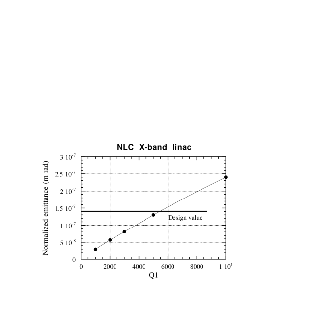
Figure 13: The normalized emittance growth vs $Q_{1}$ with $\sigma_{y}=15\ \mu$m (NLC X-band linac).

Figure 14: The normalized emittance growth vs $Q_{1}$ with $\sigma_{y}=50\mu$m (NLC S-band linac).

Machine	$l_{s}$ (m)	$N_{c}$	$f_{1}$ (GHz)	$a$ (m)	$D$ (m)	h (m)	R (m)
SBLC	6	180	4.2-4.55	0.015-0.01	0.035	0.0292	0.041
TESLA	1	9	1.7	0.035	0.115	0.0974	0.095
NLC X-band	1.8	206	15-16	0.0059-0.00414	0.00875	0.0073	0.011
NLC S-band	4	114	4.2-4.55	0.015-0.01	0.035	0.0292	0.041

Table 1: The machine parameters I.

Machine	$N_{e}$ ($\times 10^{10}$)	$s_{b}$ (m)	$E_{z}$ (MV/m)	$\sigma_{z}(\mu$m)	$N_{b}$	$Q_{1}$
SBLC	1.1	1.8	17	300	333	2000,10000
TESLA	3.63	212	25	700	1136	7000
NLC X-band	1.1	0.84	50	145	95	1000
NLC S-band	1.1	0.84	17	500	95	10000

Table 2: The machine parameters II.

Machine	$\gamma(0)$ (GeV/MeV)	$\gamma$ (GeV/MeV)	$\overline{k(s)}$ (1/m)	$\sigma_{y}$ ($\mu$m)
SBLC	3/0.511	250/0.511	1/90	100
TESLA	3/0.511	250/0.511	1/90	500
NLC X-band	10/0.511	250/0.511	1/50	15
NLC S-band	20/0.511	10/0.5111	1/20	50

Table 3: The machine parameters III.

Machine	$\epsilon^{train,numeri.}_{n,rms}$ (mrad)	$\epsilon^{train,analy.}_{n,rms}$ (mrad)	$\epsilon^{IP,design}_{n,rms}$ (mrad)
SBLC	2.3$\times 10^{-8},8.8\times 10^{-7}$	8.$\times 10^{-8},9.7\times 10^{-7}$	2.5$\times 10^{-7}$
TESLA	$\sim$2.5$\times 10^{-8}$	5.9$\times 10^{-8}$	2.5$\times 10^{-7}$
NLC X-band	-	3$\times 10^{-8}$	1.4$\times 10^{-7}$
NLC S-band	-	1.2$\times 10^{-8}$	1.4$\times 10^{-7}$

Table 4: The normalized train emittance growth.

7 Conclusion

We treat the single and multibunch emittance growths in the main linac of a linear collider in analogy to the Brownian motion of a molecule, and obtained the analytical expressions for the emittance growth due to accelerating structure misalignment errors by solving Langevin equation. As proved in this paper, the same set of formulae can be derived also by solving directly Fokker-Planck equation. Analytical results have been compared with those coming from the numerical simulations, such as SBLC and TESLA, and the agreement is quite well. As interesting applications, we give the analytical results on the estimation of the multibunch emittance growth in NLC X-band and S-band linacs.

8 Acknowledgement

It is a pleasure to discuss with J. Le Duff on the stochastic motions. I thank F. Richard for his reminding me the work of J. Perez Y Jorba on inverse multiple Touschek effect in linear colliders, and T.O. Raubenheimer for the discussion on the NLC parameters and detailed beam dynamics problems.

References

- [1] J. Gao, ”Parameter choices in linear collider designs”, LAL/RT 95-08, and ”An S-band superconducting linear collider”, Proceedings of EPAC96, Barcelona, 1996, p. 498.
- [2] A. Chao, B. Richter, and C.Y. Yao, ”Beam emittance growth caused by transverse deflecting fields in a linear accelerator”, Nucl. Instr. and Methods, 178 (1980), p. 1.
- [3] V.E. Balakin, A.V. Novokhatsky, and V.P. Simirnov, ”VLEPP: Transverse beam dynamics”, and ”Stochastic beam heating”, Proc. 12th Int. Conf. on High Energy Accelerators, Batavia, Fermilab, USA (1983), p. 119, and p. 121.
- [4] T.O. Raubenheimer, ”The generation and acceleration of low emittance flat beams for future linear colliders”, SLAC-Report-387, 1991.
- [5] J. Perez Y Jorba, ”Increase of emittance in high energy e+e- colliders by inverse multiple Touschek effect in single bunches”, Nucl. Instr. and Methods, A297 (1990), p. 31.
- [6] S. Chandrasekhar, ”Stochastic problems in physics and astronomy”, Rev. of Modern Physics, Vol. 15, No. 1 (1943), p. 1.
- [7] J. Gao, ”Analytical formulae and the scaling laws for the loss factors and the wakefields in disk-loaded periodic structures”, Nucl. Instr. and Methods, A381 (1996), p. 174.
- [8] J. Gao, “Multibunch emittance growth and its corrections in S-band linear collider”, Particle Accelerators, Vol. 49 (1995), p. 117.
- [9] R. Brinkmann, et al. (editors), ”Conceptual design of a 500 GeV e+e- linear collider with integrated X-ray laser facility”, DESY 1997-048, Vol. II, 1997.
- [10] R. Brinkmann, et al. (editors), ”Conceptual design of a 500 GeV e+e- linear collider with integrated X-ray laser facility”, DESY 1997-048, Vol. I, 1997.