Quasispecies evolution on a fitness landscape with a fluctuating peak

Abstract

A quasispecies evolving on a fitness landscape with a single peak of fluctuating height is studied. In the approximation that back mutations can be ignored, the rate equations can be solved analytically. It is shown that the error threshold on this class of dynamic landscapes is defined by the time average of the selection pressure. In the case of a periodically fluctuating fitness peak we also study the phase-shift and response amplitude of the previously documented low-pass filter effect. The special case of a small harmonic fluctuation is treated analytically.

I Introduction

Ever since Eigen’s work on replicating molecules in 1971 [1], the quasispecies concept has proven to be a very fruitful way of modeling the fundamental behavior of evolution. A quasispecies is an equilibrium distribution of closely related gene sequences, localized around one or a few sequences of high fitness. The kinetics of these simple systems has been studied in great detail, and the formulation has allowed many of the techniques of statistical physics to be applied to replicator and evolutionary systems, see for instance [1, 2, 3, 4, 5, 6, 7, 8].

The appearance in these models of an error-threshold (or error-catastrophe) as an upper bound on the mutation rate above which no effective selection can occur, has important implications for biological systems. In particular it places limits on the maintainable amounts of genetic information [1, 2] which puts restrictions on theories for the origins of life.

Until now studies of quasispecies have mainly focused on static fitness landscapes. However, many organisms in nature live in a quickly changing environment. In this paper we will study how a population responds to changes in the fitness landscape. More precisely we will study the population dynamics on a fluctuating single peaked fitness landscape. Since the full theory turns out to be impossible to solve analytically, we introduce a simple approximation that makes the rate equations analytically tractable. The expression for the error threshold is then obtained from the expression in the static case by replacing the height of the fitness peak by the time average of the height of the fluctuating peak. We also study how the phase-shift between fitness oscillations and population dynamics depends on the frequency in the case of a small harmonic fluctuation.

II Quasispecies in dynamic environments

A quasispecies consists of a population of self-replicating genomes, where each genome is represented by a sequence of bases $s_{k}$, $\left(s_{1}s_{2}\cdots s_{\nu}\right)$. We assume that the bases are binary, $s_{k}\in\{1,0\}$ and that all sequences have equal length $\nu$. Every genome is then given by a binary string $\left(011001\cdots\right)$, which also can be represented by an integer $k=\sum_{j}s_{j}2^{j}$ ($0\leq k<2^{\nu}$).

To describe how mutations affect a population we define $W_{k}^{l}$ as the probability that replication of genome $l$ gives genome $k$ as offspring. We only consider point mutations, which conserve the genome length $\nu$.

We assume that the point mutation rate $\mu=1-q$ (where $q$ is the copying accuracy per base) is constant in time and independent of the position in the genome. We can then write down an explicit expression for $W_{k}^{l}$ in terms of the copying fidelity:

$$W_{k}^{l} = \mu^{h_{kl}}q^{\nu-h_{kl}}=q^{\nu}\left(\frac{1-q}{q}\right)^{h_{kl}}$$ (1)

where $h_{kl}$ is the Hamming distance between genomes $k$ and $l$. The Hamming distance $h_{kl}$ is defined as the number of positions where the genomes $k$ and $l$ differ.

The equations that describe the dynamics of the population take a relatively simple form. Let $x_{k}$ denote the relative concentration and $A_{k}(t)$ the time-dependent fitness of genome $k$. We then obtain the following rate equations:

$$\dot{x}_{k}(t) = \sum_{l}W_{k}^{l}A_{l}(t)x_{l}(t)-e(t)x_{k}(t)$$ (2)

where $e(t)=\sum_{l}A_{l}(t)x_{l}(t)$, and the dot denotes a time derivative. The second term ensures the total normalization of the population ($\sum_{l}x_{l}(t)=1$) so that $x_{k}(t)$ describe relative concentrations.

In the classical theory introduced by Eigen and coworkers [1, 9, 10], the fitness landscape is static. The rate equations (2) can then be solved analytically by introducing a change of coordinates that makes them linear, and then solving the eigenvalue system for the matrix $W_{k}^{l}A_{l}$. The equilibrium distribution is given by the eigenvector corresponding to the largest eigenvalue.

If the fitness landscape is time-dependent, this method cannot be applied. A time-ordering problem occurs when we define exponentials of time-dependent matrices, since in general the matrix $W_{k}^{l}A_{l}(t)$ does not commute with itself at different points in time. Later in this paper we make a simple approximation that makes the rate equations one-dimensional; time-ordering is then no longer necessary.

Much of the work on quasispecies has focused on fitness landscapes with one gene sequence (the master sequence) with superior fitness, $\sigma$, compared to all other sequences. These are viewed as a background with fitness $1$. These landscapes are referred to as single peaked landscapes. The master sequence is denoted $x_{0}$. In this paper we focus on single peaked landscapes where the height of the fitness peak is time-dependent. The fitness landscape is then given by

$$A_{k}(t) = \left\{\begin{array}[]{ll}\sigma(t)&\mbox{if }k=0\\ 1&\mbox{otherwise}\end{array}\right.$$ (5)

This class of time-dependent landscapes was studied by Wilke and co-workers [11, 12]. They investigated the behavior of a periodically fluctuating single peak landscape by numerically integrating the dynamics to find the limit cycle of the concentrations for a full period.

Fig. 1 shows how the concentration of the master sequence responds to a sudden, sharp jump in its fitness. When the fitness changes it takes some time for the population to reach the new equilibrium. It is this delay that causes a phase shift between a periodically changing fitness function and the response in the concentrations. The relaxation time of the population to the appropriate equilibrium distribution depends on both the fitness values of the landscape and the mutation rate. For extremely slow and smooth changes in the fitness the population will effectively reach equilibrium at every point in time. Thus the continued existence of a quasispecies will depend on the local dynamics of the landscape. When the landscape changes quickly the population will fail to follow the changes adequately and thus responds to the landscape dynamics in a way that is typical of a low pass filter. The following section examines the fluctuating single peak landscape in some detail. In particular, we introduce an approximation that lets us find an analytic form for the relaxation time of the population, and the phase lag it introduces in a periodic landscape.

FIG. 1.: The concentration of the master sequence when the fitness peak makes a sudden jump. The fitness is given by $\sigma=10$ when $t\in\left[10,12\right]$, $\sigma=5$ otherwise. The genomic copying fidelity is given by $Q=0.7$.

III Approximate quasispecies dynamics

We now introduce a simple approximation of the model presented above. In this approximation we can solve the rate equations and find an expression for the concentration of the master sequence $x_{0}(t)$. In the limit of long chain-length ($\nu\gg 1$) we can neglect back-mutations from the background to the master sequence. This gives a simplified one-dimensional version of the rate equation of the following form:

$$\dot{x}_{0}(t) = Q\sigma(t)x_{0}(t)-e(t)x_{0}(t)$$ (6)

where $Q=q^{\nu}$ is the copying fidelity of the whole genome and $e(t)=(\sigma(t)-1)x_{0}(t)+1$.

Fig. 2 compares the concentration of the master sequence calculated by solving approximation 6 and by numerically integrating the full rate equation 2. The figure shows that the approximation is quite accurate.

FIG. 2.: The concentration of the master sequence calculated using the approximation 6 (dashed) and by numerically solving the rate equations 2 (solid). The fitness is given by $\sigma=10+5\sin(4t)$. The genomic copying fidelity is given by $Q=0.7$ and the genome length $\nu=25$.

Since this equation is one-dimensional there is no time-ordering problem and it can be solved analytically for non-periodic peak fluctuations. Equation 6 can be transformed to a linear form by introducing a new variable $y(t)=\frac{Q-x_{0}(t)}{(1-Q)x_{0}(t)}$. This gives

$$\dot{y}(t) = 1-(Q\sigma(t)-1)y(t)$$ (7)

which can be solved. Substituting back gives the concentration of the master sequence

$$x_{0}(t) = x_{0}\frac{e^{\int_{0}^{t}(Q\sigma(s)-1)ds}}{1+x_{0}\int_{0}^{t}e^{\int_{0}^{s}(Q\sigma(u)-1)du}(\sigma(s)-1)ds}$$ (8)

Since we are only interested in the long time behavior of the system we can ignore transients carrying memory from initial values. Assuming $e^{\int_{0}^{t}(Q\sigma(s)-1)ds}\gg 1$ gives

$$x_{0}(t) = \frac{Q}{1+(1-Q)\int_{0}^{t}e^{-\int_{s}^{t}(Q\sigma(u)-1)du}ds}$$ (9)

This is a generalization of the static expression for the asymptotic concentration:

$$x_{0}^{s} = \frac{Q\sigma-1}{\sigma-1}$$ (10)

On a static single peaked fitness landscape there is a phase transition in the concentration distribution when the copying fidelity decreases below a critical value [2, 13]. At high mutation rate the selective advantage of the master sequence due to its superior fitness is no longer strong enough for the gene sequences to be localized in sequence space. Instead they diffuse over the entire sequence space, and the distribution becomes approximately uniform. This is generally referred to as the error catastrophe or error threshold and is one of the main implications of the original quasispecies model. By making the same approximation as above, i.e. assuming no back-mutations onto the master sequence, the static landscape error threshold can be shown to occur when $Q=\frac{1}{\sigma}$. In other words, the transition occurs when the selective advantage of the master-sequence no longer is able to compensate for the loss of offspring due to mutations. This can also be seen from Eq. 10 which defines the stationary distribution of the master sequence in the static case.

One has to be careful when discussing the error threshold on a fluctuating peak. The fitness can, for example, slowly move from being strong enough to localize the population around the peak, to beibg so weak that the population delocalizes, and then back again. If we however consider an average over a time scale much longer than the fluctuation time of the fitness peak, a sensible definition of the error threshold can be made based on the average concentration of the master sequence. The time average of the concentrations can be found by rewriting equation 6 as differentials

$$\int\frac{dx_{0}}{x_{0}} = \int(Q\sigma(t)-1-(\sigma(t)-1)x_{0}(t))dt$$ (11)

The concentration of the master-sequence is positive. The left hand side of Eq. 11 is therefore positive and the last term in the integral, $-(\sigma(t)-1)x_{0}(t)$, on the left hand side is negative. This implies that for $x_{0}(t)$ to be positive as time goes to infinity, we must assume $\int\left(Q\sigma(t)-1\right)dt>0$. The fluctuating time dependent equivalent to the static error threshold is therefore given by

$$Q_{fc} = \frac{1}{\langle\sigma\rangle_{t}}$$ (12)

This shows that the error threshold on a fluctuating fitness peak is determined by the time average of the fitness, if the fluctuations are fast compared to the response time of the population.

Eq. 9 indicates that the response time of the system is approximately given by $(Q\sigma(t)-1)^{-1}$, i.e. the relative growth of the mastersequence compared to the background. For the time average mentioned above to be an interesting parameter the fluctuations of the fitness peak must therefore be faster than this response time; only for this kind of environmental dynamics is it sensible to talk in terms of the average concentration of the master-sequence. Thus if the fluctuations occur on a time-scale faster than the response-time of the quasispecies, then the error-threshold is defined by Eq. 12. For extremely slow changes the system will effectively be in equilibrium around the current value of the fitness. For slightly faster changes the response of the population will lag somewhat behind the changes in selective environment. In these cases it is more interesting to study the minimal concentration of the master sequence, which occurs when the fitness peak has a minimum (as we shall see later the phase-shift decreases when the fluctuation frequency decreases).

When the full replicator equations for a rapidly fluctuating peak are numerically integrated, the time-averaged quasispecies distribution displays an error catastrophe at high error rates $\mu=1-q$. In figure 3 the fitness peak fluctuates periodically with $\sigma(t)=10+5\sin(t)$. The average fitness is given by $\langle\sigma\rangle_{t}=10$ and the genome length $\nu=25$ and thus Eq. 12 predicts the error-threshold to occur at $\mu=0.088$, which agrees with the value found by numerically integrating the equations of motion directly. The analysis in this section demonstrates that by making the error tail approximation and reducing the dynamics to one-dimensional form, an analytic form exists for the error-threshold on fast moving landscapes. This one-dimensional formulation removes the need to time-order the changes in selective advantage of the landscape. This allows the integrals for the time history of the master-sequence concentration to be solved explicitly in equation 8.

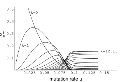
FIG. 3.: The time-averaged quasispecies distribution is shown as a function of the error rate $\mu=q-1$. The figure shows the numerical solution to the full rate equations. The fitness peak is defined as $\sigma(t)=10+5\sin(t)$ and the genome length is $\nu=25$. The error threshold is located at $\mu\approx 0.085$, corresponding to $Q_{fc}=0.109$ which can be compared to the approximate value $Q_{fc}=0.1$ predicted by Eq. 12.

IV Phase-shifts on periodic landscapes

To study how the master sequence responds to changes in the height of the fitness peak it is convenient to assume that the fluctuations are periodic. It then makes sense to speak of the amplitude of the oscillations in concentration and of the phase-shift between the concentration and the fitness. It is intuitively clear that when the fitness peak is oscillating slowly (compared to the response time $(Q\sigma(t)-1)^{-1}$) there will be a very small phase-shift; the population will have time to reach an equilibrium about every value of $\sigma(t)$. The amplitude of changes in the master-sequence concentration will, for the same reason, be as large as possible. This result, together with the time-averaging effect found in the previous section, indicates that the population responds to the driving of the environment with a low pass filter effect. In one-dimensional population genetic models this phenomenon has been noted for some time [14, 15, 16]. Wilke et al. [11] demonstrated via simulations that the same filtering occurred to quasispecies evolution on a periodically fluctuating single peak. Noting that the maxima and minima in concentration occurs when $\dot{x}_{0}=0$, we can find a relation between the phase-shift (between the concentration and fitness fluctuations), and the amplitude of the fitness fluctuations. Let $t_{xmax}$ be the time when the concentration has a maximum. Similarly the fitness is at a maximum at time $t_{\sigma max}$. Thus the phase-shift between the two is $\delta=t_{xmax}-t_{\sigma max}$. From equation 6 the condition for the maximum value of $x_{0}$ during a full cycle can be derived

$$\max_{t}(x_{0}(t)) = \frac{Q\sigma(t_{\sigma max}+\delta)-1}{\sigma(t_{\sigma max}+t_{\delta})-1}$$ (13)

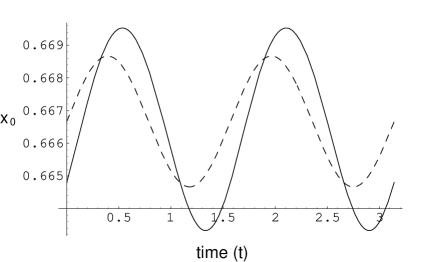
FIG. 4.: Thhe response in concentration of the master sequence (solid line) as the fitness peak oscillates according to $\sigma(t)=10+\sin(4t)$. The genomic copying fidelity is $Q=0.7$. The dashed line shows $\sigma(t)$, scaled to fit in the plot. Note the phase-shift between the fitness function and the concentration response.

In general there is no closed analytic expression for this phase-shift ($\delta$), or the response amplitude of the master-sequence concentration. When the fluctuations of the fitness peak is a small harmonic oscillation equation 13 becomes analytically tractable. For such fluctuations

$$\dot{y}(t) = 1-(Q\sigma(t)-1)y(t)$$ (14)

$$\sigma(t) = \bar{\sigma}+\epsilon\sin(\omega t)$$ (15)

From equation 9 it is reasonable to assume the solution to be of the form $y(t)=\frac{1}{Q\bar{\sigma}-1}+u(t)$, where $u(t)$ is small compared to the average. Ignoring higher order terms equation 6 can be written in terms of the perturbation $u(t)$ as

$$\dot{u}(t) = (1-Q\bar{\sigma})u(t)-\frac{\epsilon Q\sin(\omega t)}{Q\bar{\sigma}-1}$$ (16)

This differential equation can be solved to obtain

$$u(t) = -\frac{\epsilon Q}{(Q\bar{\sigma}-1)\sqrt{(Q\bar{\sigma}-1)^{2}+\omega^{2}}}\sin(\omega t-\delta)$$ (17)

$$\tan(\delta) = \frac{\omega}{Q\bar{\sigma}-1}$$ (18)

In eq. 17 and 18 transients have been ignored since they decay exponentially as $e^{-(Q\bar{\sigma}-1)t}$. Thus the frequency of the oscillations is normalized by the (average) response rate of the population $Q\bar{\sigma}-1$.

FIG. 5.: The phase shift as a function of the period $T=\frac{2\pi}{\omega}$. The dashed line is a prediction using Eq. 18 and the solid is derived by numerically solving the reate equations 2. Parameters used are $\sigma=10+\sin(\omega t)$, $Q=0.7$ and $\nu=25$.

Substituting this back into the expression for $x_{0}(t)$ gives

$$x_{0}(t) = \frac{\bar{x}}{1-\frac{\epsilon(1-Q)\sin(\omega t-\delta)}{(\bar{\sigma}-1)\sqrt{(Q\bar{\sigma}-1)^{2}+\omega^{2}}}}$$ (19)

where $\bar{x}=\frac{Q\bar{\sigma}-1}{\bar{\sigma}-1}$.

The characteristic behavior of a low pass filter is clearly shown in equation 18 and  19. As the frequency of the fluctuations increases, the amplitude of the concentration response decreases and the phase shift converges to $\frac{\pi}{2}$. Figure 4 shows how a population responds to harmonic oscillations of the fitness peak. The phase-shift makes the concentration of the mastersequence reach its maximum when the actual fitness has already decreased below maximum.

V Conclusions

In this paper we have shown that the time dynamics of a quasispecies on a fluctuating peak can be studied under the standard no back-mutation approximation. The general time ordering problem stemming from a time dependent landscape disappears since the rate equation becomes one–dimensional. We show that the time dependent equivalent to the static error threshold is determined by the time average of the fluctuations of the fitness peak. An expression for the typical response time for a population is given in terms of copying fidelity and selection pressure. We also show that for small periodic fluctuations the time dynamics of the population has a phase shift and a low pass filter amplitude response. Analytic expressions for the phase shift and the amplitude are derived in the special case of small harmonically oscillating fluctuations.

When doing this work Nigel Snoad and Martin Nilsson were supported by SFI core funding grants. N.S. would also like to acknowledge the support of Mats Nordahl at Chalmers University of Technology while preparing this manuscript. We also Mats Nordahl for valuable comments and discussions.

REFERENCES

- [1] M. Eigen. Self-organization of matter and the evolution of biological macromolecules. Naturwissenschaften, 58:465–523, 1971.
- [2] M. Eigen and P. Schuster. The hypercycle. A principle of natural self-organization. Part A: emergence of the hypercycle. Naturwissenschaften, 64:541–565, 1977.
- [3] P. Schuster. Dynamics of Molecular Evolution. Physica D, 16:100–119, 1986.
- [4] P. Schuster and K. Sigmund. Dynamics of Evolutionary Optimization. Ber. Bunsenges. Phys. Chem., 89:668–682, 1985.
- [5] I. Leuthäusser. An exact correspondence between Eigen’s evolution model and a two-dimensional Ising system. J. Chem. Phys., 84(3):1884–1885, 1986.
- [6] P. Tarazona. Error thresholds for molecular quasispecies as phase transitions: From simple landscapes to spin-glass models. Physical Review A, 45(8):6038–6050, 1992.
- [7] J. Swetina and P. Schuster. Stationary Mutant Distribution and Evolutionary Optimization. Bulletin of Mathematical Biology, 50:635–660, 1988.
- [8] M. Nowak and P. Schuster. Error thresholds of replication in finite populations: Mutation frequencies and the onset of Müller’s ratchet. J. theor. Biol., 137:375–395, 1989.
- [9] M. Eigen and P. Schuster. The hypercycle – a principle of natural selforganization. Springer, Berlin, 1979.
- [10] M. Eigen, J. McCaskill, and P. Schuster. The molecular quasispecies. Adv. Chem. Phys., 75:149–263, 1989.
- [11] C.O. Wilke, C. Ronnewinkel, and T. Martinetz. Molecular evolution in time dependent environments. In H. Lund and R. Kortmann, editors, Proc. ECAL’99, Lecture Notes in Computer Science, page 417, Heidelberg, 1999. Springer-Verlag. LANL e-print archive: physics/9904028.
- [12] C.O. Wilke, C. Ronnewinkel, and T. Martinetz. Dynamic fitness landscapes in the quasispecies model. LANL e-print archive: physics/9912012, December 1999.
- [13] J. Maynard Smith and E. Szathmáry. The Major Transitions in Evolution. W.H. Freeman, Oxford, 1995.
- [14] K. Ishii, H. Matsuda, Y. Iwasa, and A. Saskai. Evolutionarily stable mutation rate in a periodically changing environment. Genetics, 121:163–174, January 1989.
- [15] B. Charlesworth. The evolution of sex and recombination in a varying environment. J. Hered., 84:345–350, 1993.
- [16] R. Lande and S. Shannon. The role of genetic variation in adaptation and population persistence in a changing environment. Evolution, 50:434–437, 1996.