Variational–Wavelet Approach to RMS Envelope Equations

Abstract

We present applications of variational–wavelet approach to nonlinear (rational) rms envelope equations. We have the solution as a multiresolution (multiscales) expansion in the base of compactly supported wavelet basis. We give extension of our results to the cases of periodic beam motion and arbitrary variable coefficients. Also we consider more flexible variational method which is based on biorthogonal wavelet approach.

1 Introduction

In this paper we consider the applications of a new numerical-analytical technique which is based on the methods of local nonlinear Fourier analysis or Wavelet analysis to the nonlinear beam/accelerator physics problems related to root-mean-square (rms) envelope dynamics [1]. Such approach may be useful in all models in which it is possible and reasonable to reduce all complicated problems related with statistical distributions to the problems described by systems of nonlinear ordinary/partial differential equations. In this paper we consider approach based on the second moments of the distribution functions for the calculation of evolution of rms envelope of a beam.

The rms envelope equations are the most useful for analysis of the beam self–forces (space–charge) effects and also allow to consider both transverse and longitudinal dynamics of space-charge-dominated relativistic high–bright ness axisymmetric/asymmetric beams, which under short laser pulse–driven radio-frequency photoinjectors have fast transition from nonrelativistic to relativistic regime [2]-[3].

From the formal point of view we may consider rms envelope equations after straightforward transformations to standard Cauchy form as a system of nonlinear differential equations which are not more than rational (in dynamical variables). Such rational type of nonlinearities allow us to consider some extension of results from [4]-[12], which are based on application of wavelet analysis technique to variational formulation of initial nonlinear problem.

Wavelet analysis is a relatively novel set of mathematical methods, which gives us a possibility to work with well-localized bases in functional spaces and give for the general type of operators (differential, integral, pseudodifferential) in such bases the maximum sparse forms.

An example of such type of basis is demonstrated on Fig. 1.

Our approach in this paper is based on the generalization [13] of variational-wavelet approach from [4]-[12], which allows us to consider not only polynomial but rational type of nonlinearities.

So, our variational-multiresolution approach gives us possibility to construct explicit numerical-analytical solution for the following systems of nonlinear differential equations

$$\dot{z}=R(z,t)\quad\mbox{or}\quad Q(z,t)\dot{z}=P(z,t),$$ (1)

where $z(t)=(z_{1}(t),...,z_{n}(t))$ is the vector of dynamical variables $z_{i}(t)$,

$R(z,t)$ is not more than rational function of z,

$P(z,t),Q(z,t)$ are not more than polynomial functions of z and P,Q,R have arbitrary dependence of time.

The solution has the following form

$$z(t)=z_{N}^{slow}(t)+\sum_{j\geq N}z_{j}(\omega_{j}t),\quad\omega_{j}\sim 2^{j}$$ (2)

which corresponds to the full multiresolution expansion in all time scales. Formula (2) gives us expansion into a slow part $z_{N}^{slow}$ and fast oscillating parts for arbitrary N. So, we may move from coarse scales of resolution to the finest one for obtaining more detailed information about our dynamical process. The first term in the RHS of equation (2) corresponds on the global level of function space decomposition to resolution space and the second one to detail space. In this way we give contribution to our full solution from each scale of resolution or each time scale (detailed description we give in part 3.2 and numerical illustration in part 7 below). The same is correct for the contribution to power spectral density (energy spectrum): we can take into account contributions from each level/scale of resolution.

In part 2 we describe the different forms of rms equations. Starting in part 3.1 from variational formulation of initial dynamical problem we construct via multiresolution analysis (3.2) explicit representation for all dynamical variables in the base of compactly supported (Daubechies) wavelets. Our solutions (3.3) are parametrized by solutions of a number of reduced algebraical problems one from which is nonlinear with the same degree of nonlinearity and the rest are the linear problems which correspond to particular method of calculation of scalar products of functions from wavelet bases and their derivatives. Then we consider further extension of our previous results. In part 4 we consider modification of our construction to the periodic case, in part 5 we consider generalization of our approach to variational formulation in the biorthogonal bases of compactly supported wavelets and in part 6 to the case of variable coefficients. In part 7 we consider results of numerical calculations.

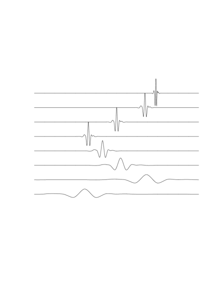
Figure 1: Wavelets at different scales and locations.

2 RMS Equations

Below we consider a number of different forms of RMS envelope equations, which are from the formal point of view not more than nonlinear differential equations with rational nonlinearities and variable coefficients. Let $f(x_{1},x_{2})$ be the distribution function which gives full information about noninteracting ensemble of beam particles regarding to trace space or transverse phase coordinates $(x_{1},x_{2})$. Then (n,m) moments are:

$$\int\int x_{1}^{n}x_{2}^{m}f(x_{1},x_{2})\mathrm{d}x_{1}\mathrm{d}x_{2}$$ (3)

The (0,0) moment gives normalization condition on the distribution. The (1,0) and (0,1) moments vanish when a beam is aligned to its axis. Then we may extract the first nontrivial bit of ‘dynamical information’ from the second moments

$$\sigma_{x_{1}}^{2} = <x_{1}^{2}>=\int\int x_{1}^{2}f(x_{1},x_{2})\mathrm{d}x_{1}\mathrm{d}x_{2}$$

$$\sigma_{x_{2}}^{2} = <x_{2}^{2}>=\int\int x_{2}^{2}f(x_{1},x_{2})\mathrm{d}x_{1}\mathrm{d}x_{2}$$ (4)

$$\sigma_{x_{1}x_{2}}^{2} = <x_{1}x_{2}>=\int\int x_{1}x_{2}f(x_{1},x_{2})\mathrm{d}x_{1}\mathrm{d}x_{2}$$

RMS emittance ellipse is given by

$$\varepsilon^{2}_{x,rms}=<x_{1}^{2}><x_{2}^{2}>-<x_{1}x_{2}>^{2}$$ (5)

Expressions for twiss parameters are also based on the second moments.

We will consider the following particular cases of rms envelope equations, which described evolution of the moments (4) ([1]-[3] for full designation):

for asymmetric beams we have the system of two envelope equations of the second order for $\sigma_{x_{1}}$ and $\sigma_{x_{2}}$:

$$\sigma^{{}^{\prime\prime}}_{x_{1}}+\sigma^{{}^{\prime}}_{x_{1}}\frac{\gamma^{\prime}}{\gamma}+\Omega^{2}_{x_{1}}\left(\frac{\gamma^{\prime}}{\gamma}\right)^{2}\sigma_{x_{1}} = \frac{I}{I_{0}(\sigma_{x_{1}}+\sigma_{x_{2}})\gamma^{3}}+\frac{\varepsilon^{2}_{nx_{1}}}{\sigma_{x_{1}}^{3}\gamma^{2}},$$

$$\sigma^{{}^{\prime\prime}}_{x_{2}}+\sigma^{{}^{\prime}}_{x_{2}}\frac{\gamma^{\prime}}{\gamma}+\Omega^{2}_{x_{2}}\left(\frac{\gamma^{\prime}}{\gamma}\right)^{2}\sigma_{x_{2}} = \frac{I}{I_{0}(\sigma_{x_{1}}+\sigma_{x_{2}})\gamma^{3}}+\frac{\varepsilon^{2}_{nx_{2}}}{\sigma_{x_{2}}^{3}\gamma^{2}}$$ (6)

the envelope equation for an axisymmetric beam is

$$\sigma^{{}^{\prime\prime}}+\sigma^{{}^{\prime}}\frac{\gamma^{\prime}}{\gamma}+\Omega^{2}\left(\frac{\gamma^{\prime}}{\gamma}\right)^{2}\sigma=\frac{k_{s}}{\sigma\gamma^{3}}+\frac{\varepsilon^{2}_{n,th}}{\sigma^{3}\gamma^{2}}$$ (7)

Also we have related Lawson’s equation for evolution of the rms envelope in the paraxial limit, which governs evolution of cylindrical symmetric envelope under external linear focusing channel of strenghts $K_{r}$:

$$\sigma^{{}^{\prime\prime}}+\sigma^{{}^{\prime}}\left(\frac{\gamma^{\prime}}{\beta^{2}\gamma}\right)+K_{r}\sigma=\frac{k_{s}}{\sigma\beta^{3}\gamma^{3}}+\frac{\varepsilon^{2}_{n}}{\sigma^{3}\beta^{2}\gamma^{2}},$$

where

$$K_{r}\equiv-F_{r}/r\beta^{2}\gamma mc^{2},\ \ \ \beta\equiv\nu_{b}/c=\sqrt{1-\gamma^{-2}}$$

After transformations to Cauchy form we can see that all this equations from the formal point of view are not more than ordinary differential equations with rational nonlinearities and variable coefficients and correspond to the form (1) (also,we may consider regimes in which $\gamma$, $\gamma^{\prime}$ are not fixed functions/constants but satisfy some additional differential constraint/equation, but this case does not change our general approach).

3 Rational Dynamics

The first main part of our consideration is some variational approach to this problem, which reduces initial problem to the problem of solution of functional equations at the first stage and some algebraical problems at the second stage. We have the solution in a compactly supported wavelet basis. Multiresolution expansion is the second main part of our construction. The solution is parameterized by solutions of two reduced algebraical problems, one is nonlinear and the second are some linear problems, which are obtained from one of the next wavelet constructions: the method of Connection Coefficients (CC), Stationary Subdivision Schemes (SSS).

3.1 Variational Method

Our problems may be formulated as the systems of ordinary differential equations

$$Q_{i}(x)\frac{\mathrm{d}x_{i}}{\mathrm{d}t}=P_{i}(x,t),\quad x=(x_{1},...,x_{n}),$$ (8)

$$\quad i=1,...,n,\quad\max_{i}deg\ P_{i}=p,\quad\max_{i}deg\ Q_{i}=q$$

with fixed initial conditions $x_{i}(0)$, where $P_{i},Q_{i}$ are not more than polynomial functions of dynamical variables $x_{j}$ and have arbitrary dependence of time. Because of time dilation we can consider only next time interval: $0\leq t\leq 1$. Let us consider a set of functions

$$\Phi_{i}(t)=x_{i}\frac{\mathrm{d}}{\mathrm{d}t}(Q_{i}y_{i})+P_{i}y_{i}$$ (9)

and a set of functionals

$$F_{i}(x)=\int_{0}^{1}\Phi_{i}(t)dt-Q_{i}x_{i}y_{i}\mid^{1}_{0},$$ (10)

where $y_{i}(t)\ (y_{i}(0)=0)$ are dual (variational) variables. It is obvious that the initial system and the system

$$F_{i}(x)=0$$ (11)

are equivalent. Of course, we consider such $Q_{i}(x)$ which do not lead to the singular problem with $Q_{i}(x)$, when $t=0$ or $t=1$, i.e. $Q_{i}(x(0)),Q_{i}(x(1))\neq\infty$.

In part 5 we consider more general approach, which is based on possibility taking into account underlying symplectic structure and on more useful and flexible analytical approach, related to bilinear structure of initial functional. Now we consider formal expansions for $x_{i},y_{i}$:

$$x_{i}(t)=x_{i}(0)+\sum_{k}\lambda_{i}^{k}\varphi_{k}(t)\quad y_{j}(t)=\sum_{r}\eta_{j}^{r}\varphi_{r}(t),$$ (12)

where $\varphi_{k}(t)$ are useful basis functions of some functional space ($L^{2},L^{p}$, Sobolev, etc) corresponding to concrete problem and because of initial conditions we need only $\varphi_{k}(0)=0$.

$$\lambda=\{\lambda_{i}\}=\{\lambda^{r}_{i}\}=(\lambda_{i}^{1},\lambda_{i}^{2},...,\lambda_{i}^{N}),\quad r=1,...,N,\quad i=1,...,n,$$ (13)

where the lower index i corresponds to expansion of dynamical variable with index i, i.e. $x_{i}$ and the upper index $r$ corresponds to the numbers of terms in the expansion of dynamical variables in the formal series. Then we put (12) into the functional equations (11) and as result we have the following reduced algebraical system of equations on the set of unknown coefficients $\lambda_{i}^{k}$ of expansions (12):

$$L(Q_{ij},\lambda,\alpha_{I})=M(P_{ij},\lambda,\beta_{J}),$$ (14)

where operators L and M are algebraization of RHS and LHS of initial problem (8), where $\lambda$ (13) are unknowns of reduced system of algebraical equations (RSAE)(14).

$Q_{ij}$ are coefficients (with possible time dependence) of LHS of initial system of differential equations (8) and as consequence are coefficients of RSAE.

$P_{ij}$ are coefficients (with possible time dependence) of RHS of initial system of differential equations (8) and as consequence are coefficients of RSAE.

$I=(i_{1},...,i_{q+2}),\ J=(j_{1},...,j_{p+1})$ are multiindexes, by which are labelled $\alpha_{I}$ and $\beta_{I}$ — other coefficients of RSAE (14):

$$\beta_{J}=\{\beta_{j_{1}...j_{p+1}}\}=\int\prod_{1\leq j_{k}\leq p+1}\varphi_{j_{k}},$$ (15)

where p is the degree of polinomial operator P (8)

$$\alpha_{I}=\{\alpha_{i_{1}}...\alpha_{i_{q+2}}\}=\sum_{i_{1},...,i_{q+2}}\int\varphi_{i_{1}}...\dot{\varphi_{i_{s}}}...\varphi_{i_{q+2}},$$ (16)

where q is the degree of polynomial operator Q (8), $i_{\ell}=(1,...,q+2)$, $\dot{\varphi_{i_{s}}}=\mathrm{d}\varphi_{i_{s}}/\mathrm{d}t$.

Now, when we solve RSAE (14) and determine unknown coefficients from formal expansion (12) we therefore obtain the solution of our initial problem. It should be noted if we consider only truncated expansion (12) with N terms then we have from (14) the system of $N\times n$ algebraical equations with degree $\ell=max\{p,q\}$ and the degree of this algebraical system coincides with degree of initial differential system. So, we have the solution of the initial nonlinear (rational) problem in the form

$$x_{i}(t)=x_{i}(0)+\sum_{k=1}^{N}\lambda_{i}^{k}X_{k}(t),$$ (17)

where coefficients $\lambda_{i}^{k}$ are roots of the corresponding reduced algebraical (polynomial) problem RSAE (14). Consequently, we have a parametrization of solution of initial problem by solution of reduced algebraical problem (14). The first main problem is a problem of computations of coefficients $\alpha_{I}$ (16), $\beta_{J}$ (15) of reduced algebraical system. As we will see, these problems may be explicitly solved in wavelet approach.

Next we consider the construction of explicit time solution for our problem. The obtained solutions are given in the form (17), where $X_{k}(t)$ are basis functions and $\lambda_{k}^{i}$ are roots of reduced system of equations. In our first wavelet case $X_{k}(t)$ are obtained via multiresolution expansions and represented by compactly supported wavelets and $\lambda_{k}^{i}$ are the roots of corresponding general polynomial system (14) with coefficients, which are given by CC or SSS constructions. According to the variational method to give the reduction from differential to algebraical system of equations we need compute the objects $\alpha_{I}$ and $\beta_{J}$.

3.2 Wavelet Framework

Our constructions are based on multiresolution approach. Because affine group of translation and dilations is inside the approach, this method resembles the action of a microscope. We have contribution to final result from each scale of resolution from the whole infinite scale of spaces. More exactly, the closed subspace $V_{j}(j\in{\bf Z})$ corresponds to level j of resolution, or to scale j. We consider a r-regular multiresolution analysis of $L^{2}({\bf R}^{n})$ (of course, we may consider any different functional space) which is a sequence of increasing closed subspaces $V_{j}$:

$$...V_{-2}\subset V_{-1}\subset V_{0}\subset V_{1}\subset V_{2}\subset...$$ (18)

satisfying the following properties:

$$\displaystyle\bigcap_{j\in{\bf Z}}V_{j}=0,\quad\overline{\displaystyle\bigcup_{j\in{\bf Z}}}V_{j}=L^{2}({\bf R}^{n}),$$

$$f(x)\in V_{j}<=>f(2x)\in V_{j+1},$$

$$f(x)\in V_{0}<=>f(x-k)\in V_{0},\quad,\forall k\in{\bf Z}^{n}.$$ (19)

There exists a function $\varphi\in V_{0}$ such that {${\varphi_{0,k}(x)=\varphi(x-k)},k\in{\bf Z}^{n}$} forms a Riesz basis for $V_{0}$.

The function $\varphi$ is regular and localized: $\varphi$ is $C^{r-1},\quad\varphi^{(r-1)}$ is almost everywhere differentiable and for almost every $x\in{\bf R}^{n}$, for every integer $\alpha\leq r$ and for all integer p there exists constant $C_{p}$ such that

$$\mid\partial^{\alpha}\varphi(x)\mid\leq C_{p}(1+|x|)^{-p}$$ (20)

Let $\varphi(x)$ be a scaling function, $\psi(x)$ is a wavelet function and $\varphi_{i}(x)=\varphi(x-i)$. Scaling relations that define $\varphi,\psi$ are

$$\varphi(x) = \sum\limits^{N-1}_{k=0}a_{k}\varphi(2x-k)=\sum\limits^{N-1}_{k=0}a_{k}\varphi_{k}(2x),$$ (21)

$$\psi(x) = \sum\limits^{N-2}_{k=-1}(-1)^{k}a_{k+1}\varphi(2x+k).$$ (22)

Let indices $\ell,j$ represent translation and scaling, respectively and

$$\varphi_{jl}(x)=2^{j/2}\varphi(2^{j}x-\ell)$$ (23)

then the set $\{\varphi_{j,k}\},{k\in{\bf Z}^{n}}$ forms a Riesz basis for $V_{j}$. The wavelet function $\psi$ is used to encode the details between two successive levels of approximation. Let $W_{j}$ be the orthonormal complement of $V_{j}$ with respect to $V_{j+1}$:

$$V_{j+1}=V_{j}\bigoplus W_{j}.$$ (24)

Then just as $V_{j}$ is spanned by dilation and translations of the scaling function, so are $W_{j}$ spanned by translations and dilation of the mother wavelet $\psi_{jk}(x)$, where

$$\psi_{jk}(x)=2^{j/2}\psi(2^{j}x-k).$$ (25)

All expansions which we used are based on the following properties:

$$\{\psi_{jk}\},\quad j,k\in{\bf Z}\quad\mbox{is a Hilbertian basis of }L^{2}({\bf R})$$

$$\{\varphi_{jk}\}_{j\geq 0,k\in{\bf Z}}\quad\mbox{is an orthonormal basis for}L^{2}({\bf R}),$$

$$L^{2}({\bf R})=\overline{V_{0}\displaystyle\bigoplus^{\infty}_{j=0}W_{j}},$$ (26)

or

$$\{\varphi_{0,k},\psi_{j,k}\}_{j\geq 0,k\in{\bf Z}}\quad\mbox{is an orthonormal basis for}L^{2}({\bf R}).$$

3.3 Wavelet Computations

Now we give construction for computations of objects (17),(18) in the wavelet case. We use compactly supported wavelet basis: orthonormal basis for functions in $L^{2}({\bf R})$.

Let be $f:{\bf R}\longrightarrow{\bf C}$ and the wavelet expansion is

$$f(x)=\sum\limits_{\ell\in{\bf Z}}c_{\ell}\varphi_{\ell}(x)+\sum\limits_{j=0}^{\infty}\sum\limits_{k\in{\bf Z}}c_{jk}\psi_{jk}(x)$$ (27)

If in formulae (29) $c_{jk}=0$ for $j\geq J$, then $f(x)$ has an alternative expansion in terms of dilated scaling functions only $f(x)=\sum\limits_{\ell\in{\bf Z}}c_{J\ell}\varphi_{J\ell}(x)$. This is a finite wavelet expansion, it can be written solely in terms of translated scaling functions. Also we have the shortest possible support: scaling function $DN$ (where $N$ is even integer) will have support $[0,N-1]$ and $N/2$ vanishing moments. There exists $\lambda>0$ such that $DN$ has $\lambda N$ continuous derivatives; for small $N,\lambda\geq 0.55$. To solve our second associated linear problem we need to evaluate derivatives of $f(x)$ in terms of $\varphi(x)$. Let be $\varphi^{n}_{\ell}=\mathrm{d}^{n}\varphi_{\ell}(x)/\mathrm{d}x^{n}$. We consider computation of the wavelet - Galerkin integrals. Let $f^{d}(x)$ be d-derivative of function $f(x)$, then we have $f^{d}(x)=\sum_{\ell}c_{l}\varphi_{\ell}^{d}(x)$, and values $\varphi_{\ell}^{d}(x)$ can be expanded in terms of $\varphi(x)$

$$\phi_{\ell}^{d}(x) = \sum\limits_{m}\lambda_{m}\varphi_{m}(x),$$ (28)

$$\lambda_{m} = \int\limits_{-\infty}^{\infty}\varphi_{\ell}^{d}(x)\varphi_{m}(x)\mathrm{d}x,$$

where $\lambda_{m}$ are wavelet-Galerkin integrals. The coefficients $\lambda_{m}$ are 2-term connection coefficients. In general we need to find $(d_{i}\geq 0)$

$$\Lambda^{d_{1}d_{2}...d_{n}}_{\ell_{1}\ell_{2}...\ell_{n}}=\int\limits_{-\infty}^{\infty}\prod\varphi^{d_{i}}_{\ell_{i}}(x)dx$$ (29)

For Riccati case we need to evaluate two and three connection coefficients

$$\Lambda_{\ell}^{d_{1}d_{2}}=\int^{\infty}_{-\infty}\varphi^{d_{1}}(x)\varphi_{\ell}^{d_{2}}(x)dx,\quad\Lambda^{d_{1}d_{2}d_{3}}=\int\limits_{-\infty}^{\infty}\varphi^{d_{1}}(x)\varphi_{\ell}^{d_{2}}(x)\varphi^{d_{3}}_{m}(x)dx$$ (30)

According to CC method [14] we use the next construction. When $N$ in scaling equation is a finite even positive integer the function $\varphi(x)$ has compact support contained in $[0,N-1]$. For a fixed triple $(d_{1},d_{2},d_{3})$ only some $\Lambda_{\ell m}^{d_{1}d_{2}d_{3}}$ are nonzero: $2-N\leq\ell\leq N-2,\quad 2-N\leq m\leq N-2,\quad|\ell-m|\leq N-2$. There are $M=3N^{2}-9N+7$ such pairs $(\ell,m)$. Let $\Lambda^{d_{1}d_{2}d_{3}}$ be an M-vector, whose components are numbers $\Lambda^{d_{1}d_{2}d_{3}}_{\ell m}$. Then we have the first reduced algebraical system : $\Lambda$ satisfy the system of equations $(d=d_{1}+d_{2}+d_{3})$

$$A\Lambda^{d_{1}d_{2}d_{3}}=2^{1-d}\Lambda^{d_{1}d_{2}d_{3}},\qquad A_{\ell,m;q,r}=\sum\limits_{p}a_{p}a_{q-2\ell+p}a_{r-2m+p}$$ (31)

By moment equations we have created a system of $M+d+1$ equations in $M$ unknowns. It has rank $M$ and we can obtain unique solution by combination of LU decomposition and QR algorithm. The second reduced algebraical system gives us the 2-term connection coefficients:

$$A\Lambda^{d_{1}d_{2}}=2^{1-d}\Lambda^{d_{1}d_{2}},\quad d=d_{1}+d_{2},\quad A_{\ell,q}=\sum\limits_{p}a_{p}a_{q-2\ell+p}$$ (32)

For nonquadratic case we have analogously additional linear problems for objects (31). Solving these linear problems we obtain the coefficients of nonlinear algebraical system (16) and after that we obtain the coefficients of wavelet expansion (19). As a result we obtained the explicit time solution of our problem in the base of compactly supported wavelets. We use for modelling D6, D8, D10 functions and programs RADAU and DOPRI for testing.

In the following we consider extension of this approach to the case of periodic boundary conditions, the case of presence of arbitrary variable coefficients and more flexible biorthogonal wavelet approach.

4 Variational Wavelet Approach for Periodic Trajectories

We start with extension of our approach to the case of periodic trajectories. The equations of motion corresponding to our problems may be formulated as a particular case of the general system of ordinary differential equations ${dx_{i}}/{dt}=f_{i}(x_{j},t)$, $(i,j=1,...,n)$, $0\leq t\leq 1$, where $f_{i}$ are not more than rational functions of dynamical variables $x_{j}$ and have arbitrary dependence of time but with periodic boundary conditions. According to our variational approach we have the solution in the following form

$$x_{i}(t)=x_{i}(0)+\sum_{k}\lambda_{i}^{k}\varphi_{k}(t),\qquad x_{i}(0)=x_{i}(1),$$ (33)

where $\lambda_{i}^{k}$ are again the roots of reduced algebraical systems of equations with the same degree of nonlinearity and $\varphi_{k}(t)$ corresponds to useful type of wavelet bases (frames). It should be noted that coefficients of reduced algebraical system are the solutions of additional linear problem and also depend on particular type of wavelet construction and type of bases.

This linear problem is our second reduced algebraical problem. We need to find in general situation objects

$$\Lambda^{d_{1}d_{2}...d_{n}}_{\ell_{1}\ell_{2}...\ell_{n}}=\int\limits_{-\infty}^{\infty}\prod\varphi^{d_{i}}_{\ell_{i}}(x)\mathrm{d}x,$$ (34)

but now in the case of periodic boundary conditions. Now we consider the procedure of their calculations in case of periodic boundary conditions in the base of periodic wavelet functions on the interval [0,1] and corresponding expansion (35) inside our variational approach. Periodization procedure gives us

$$\hat{\varphi}_{j,k}(x) \equiv \sum_{\ell\in Z}\varphi_{j,k}(x-\ell)$$ (35)

$$\hat{\psi}_{j,k}(x) = \sum_{\ell\in Z}\psi_{j,k}(x-\ell)$$

So, $\hat{\varphi},\hat{\psi}$ are periodic functions on the interval [0,1]. Because $\varphi_{j,k}=\varphi_{j,k^{\prime}}$ if $k=k^{\prime}\mathrm{mod}(2^{j})$, we may consider only $0\leq k\leq 2^{j}$ and as consequence our multiresolution has the form $\displaystyle\bigcup_{j\geq 0}\hat{V}_{j}=L^{2}[0,1]$ with $\hat{V}_{j}=\mathrm{span}\{\hat{\varphi}_{j,k}\}^{2j-1}_{k=0}$ [15]. Integration by parts and periodicity gives useful relations between objects (36) in particular quadratic case $(d=d_{1}+d_{2})$:

$$\Lambda^{d_{1},d_{2}}_{k_{1},k_{2}}=(-1)^{d_{1}}\Lambda^{0,d_{2}+d_{1}}_{k_{1},k_{2}},\Lambda^{0,d}_{k_{1},k_{2}}=\Lambda^{0,d}_{0,k_{2}-k_{1}}\equiv\Lambda^{d}_{k_{2}-k_{1}}$$ (36)

So, any 2-tuple can be represent by $\Lambda^{d}_{k}$. Then our second additional linear problem is reduced to the eigenvalue problem for $\{\Lambda^{d}_{k}\}_{0\leq k\leq 2^{j}}$ by creating a system of $2^{j}$ homogeneous relations in $\Lambda^{d}_{k}$ and inhomogeneous equations. So, if we have dilation equation in the form $\varphi(x)=\sqrt{2}\sum_{k\in Z}h_{k}\varphi(2x-k)$, then we have the following homogeneous relations

$$\Lambda^{d}_{k}=2^{d}\sum_{m=0}^{N-1}\sum_{\ell=0}^{N-1}h_{m}h_{\ell}\Lambda^{d}_{\ell+2k-m},$$ (37)

or in such form $A\lambda^{d}=2^{d}\lambda^{d}$, where $\lambda^{d}=\{\Lambda^{d}_{k}\}_{0\leq k\leq 2^{j}}$. Inhomogeneous equations are:

$$\sum_{\ell}M_{\ell}^{d}\Lambda^{d}_{\ell}=d!2^{-j/2},$$ (38)

where objects $M_{\ell}^{d}(|\ell|\leq N-2)$ can be computed by recursive procedure

$$M_{\ell}^{d}=2^{-j(2d+1)/2}\tilde{M_{\ell}^{d}},\quad\tilde{M_{\ell}^{k}}=<x^{k},\varphi_{0,\ell}>=\sum_{j=0}^{k}{k\choose j}n^{k-j}M_{0}^{j},\quad\tilde{M_{0}^{\ell}}=1.$$ (39)

So, we reduced our last problem to standard linear algebraical problem. Then we use the same methods as in part 3.3. As a result we obtained for closed trajectories of orbital dynamics the explicit time solution (35) in the base of periodized wavelets (37).

5 Variational Approach in Biorthogonal
Wavelet Bases

Now we consider further generalization of our variational wavelet approach. Because integrand of variational functionals is represented by bilinear form (scalar product) it seems more reasonable to consider wavelet constructions [16] which take into account all advantages of this structure.

The action functional for loops in the phase space is

$$F(\gamma)=\displaystyle\int_{\gamma}pdq-\int_{0}^{1}H(t,\gamma(t))dt$$ (40)

The critical points of $F$ are those loops $\gamma$, which solve the Hamiltonian equations associated with the Hamiltonian $H$ and hence are periodic orbits.

Let us consider the loop space $\Omega=C^{\infty}(S^{1},R^{2n})$, where $S^{1}=R/{\bf Z}$, of smooth loops in $R^{2n}$. Let us define a function $\Phi:\Omega\to R$ by setting

$$\Phi(x)=\displaystyle\int_{0}^{1}\frac{1}{2}<-J\dot{x},x>dt-\int_{0}^{1}H(x(t))dt,\quad x\in\Omega$$ (41)

The critical points of $\Phi$ are the periodic solutions of $\dot{x}=X_{H}(x)$. Computing the derivative at $x\in\Omega$ in the direction of $y\in\Omega$, we find

$$\Phi^{\prime}(x)(y)=\frac{d}{d\epsilon}\Phi(x+\epsilon y)|_{\epsilon=0}=\displaystyle\int_{0}^{1}<-J\dot{x}-\bigtriangledown H(x),y>dt$$ (42)

Consequently, $\Phi^{\prime}(x)(y)=0$ for all $y\in\Omega$ iff the loop $x$ satisfies the equation

$$-J\dot{x}(t)-\bigtriangledown H(x(t))=0,$$ (43)

i.e. $x(t)$ is a solution of the Hamiltonian equations, which also satisfies $x(0)=x(1)$, i.e. periodic of period 1.

But now we need to take into account underlying bilinear structure via wavelets.

We started with two hierarchical sequences of approximations spaces [16]:

$$\dots V_{-2}\subset V_{-1}\subset V_{0}\subset V_{1}\subset V_{2}\dots,\qquad\dots\widetilde{V}_{-2}\subset\widetilde{V}_{-1}\subset\widetilde{V}_{0}\subset\widetilde{V}_{1}\subset\widetilde{V}_{2}\dots,$$

and as usually, $W_{0}$ is complement to $V_{0}$ in $V_{1}$, but now not necessarily orthogonal complement. New orthogonality conditions have now the following form:

$$\widetilde{W}_{0}\perp V_{0},\qquad W_{0}\perp\widetilde{V}_{0},\qquad V_{j}\perp\widetilde{W}_{j},\qquad\widetilde{V}_{j}\perp W_{j}$$ (44)

translates of $\psi$ $\mathrm{span}$ $W_{0}$, translates of $\tilde{\psi}\quad\mathrm{span}\quad\widetilde{W}_{0}$. Biorthogonality conditions are

$$<\psi_{jk},\tilde{\psi}_{j^{\prime}k^{\prime}}>=\int^{\infty}_{-\infty}\psi_{jk}(x)\tilde{\psi}_{j^{\prime}k^{\prime}}(x)\mathrm{d}x=\delta_{kk^{\prime}}\delta_{jj^{\prime}},$$ (45)

where $\psi_{jk}(x)=2^{j/2}\psi(2^{j}x-k)$. Functions $\varphi(x),\tilde{\varphi}(x-k)$ form dual pair:

$$<\varphi(x-k),\tilde{\varphi}(x-\ell)>=\delta_{kl},\quad<\varphi(x-k),\tilde{\psi}(x-\ell)>=0\quad\mbox{for}\quad\forall k,\ \forall\ell.$$ (46)

Functions $\varphi,\tilde{\varphi}$ generate a multiresolution analysis. $\varphi(x-k)$, $\psi(x-k)$ are synthesis functions, $\tilde{\varphi}(x-\ell)$, $\tilde{\psi}(x-\ell)$ are analysis functions. Synthesis functions are biorthogonal to analysis functions. Scaling spaces are orthogonal to dual wavelet spaces. Two multiresolutions are intertwining $V_{j}+W_{j}=V_{j+1},\quad\widetilde{V}_{j}+\widetilde{W}_{j}=\widetilde{V}_{j+1}$. These are direct sums but not orthogonal sums.

So, our representation for solution has now the form

$$f(t)=\sum_{j,k}\tilde{b}_{jk}\psi_{jk}(t),$$ (47)

where synthesis wavelets are used to synthesize the function. But $\tilde{b}_{jk}$ come from inner products with analysis wavelets. Biorthogonality yields

$$\tilde{b}_{\ell m}=\int f(t)\tilde{\psi}_{\ell m}(t)\mathrm{d}t.$$ (48)

So, now we can introduce this more complicated construction into our variational approach. We have modification only on the level of computing coefficients of reduced nonlinear algebraical system. This new construction is more flexible. Biorthogonal point of view is more stable under the action of large class of operators while orthogonal (one scale for multiresolution) is fragile, all computations are much more simpler and we accelerate the rate of convergence. In all types of (Hamiltonian) calculation, which are based on some bilinear structures (symplectic or Poissonian structures, bilinear form of integrand in variational integral) this framework leads to greater success.

6 Variable Coefficients

In the case when we have situation when our problem is described by a system of nonlinear (rational) differential equations, we need to consider extension of our previous approach which can take into account any type of variable coefficients (periodic, regular or singular). We can produce such approach if we add in our construction additional refinement equation, which encoded all information about variable coefficients [17]. According to our variational approach we need to compute integrals of the form

$$\int_{D}b_{ij}(t)(\varphi_{1})^{d_{1}}(2^{m}t-k_{1})(\varphi_{2})^{d_{2}}(2^{m}t-k_{2})\mathrm{d}x,$$ (49)

where now $b_{ij}(t)$ are arbitrary functions of time, where trial functions $\varphi_{1},\varphi_{2}$ satisfy a refinement equations:

$$\varphi_{i}(t)=\sum_{k\in{\bf Z}}a_{ik}\varphi_{i}(2t-k)$$ (50)

If we consider all computations in the class of compactly supported wavelets then only a finite number of coefficients do not vanish. To approximate the non-constant coefficients, we need choose a different refinable function $\varphi_{3}$ along with some local approximation scheme

$$(B_{\ell}f)(x):=\sum_{\alpha\in{\bf Z}}F_{\ell,k}(f)\varphi_{3}(2^{\ell}t-k),$$ (51)

where $F_{\ell,k}$ are suitable functionals supported in a small neighborhood of $2^{-\ell}k$ and then replace $b_{ij}$ in (49) by $B_{\ell}b_{ij}(t)$. In particular case one can take a characteristic function and can thus approximate non-smooth coefficients locally. To guarantee sufficient accuracy of the resulting approximation to (49) it is important to have the flexibility of choosing $\varphi_{3}$ different from $\varphi_{1},\varphi_{2}$. In the case when D is some domain, we can write

$$b_{ij}(t)\mid_{D}=\sum_{0\leq k\leq 2^{\ell}}b_{ij}(t)\chi_{D}(2^{\ell}t-k),$$ (52)

where $\chi_{D}$ is characteristic function of D. So, if we take $\varphi_{4}=\chi_{D}$, which is again a refinable function, then the problem of computation of (49) is reduced to the problem of calculation of integral

$$H(k_{1},k_{2},k_{3},k_{4})=H(k)=$$ (53)

$$\int_{{\bf R}^{s}}\varphi_{4}(2^{j}t-k_{1})\varphi_{3}(2^{\ell}t-k_{2})\varphi_{1}^{d_{1}}(2^{r}t-k_{3})\varphi_{2}^{d_{2}}(2^{s}t-k_{4})\mathrm{d}x$$

The key point is that these integrals also satisfy some sort of refinement equation [17]:

$$2^{-|\mu|}H(k)=\sum_{\ell\in{\bf Z}}b_{2k-\ell}H(\ell),\qquad\mu=d_{1}+d_{2}.$$ (54)

This equation can be interpreted as the problem of computing an eigenvector. Thus, we reduced the problem of extension of our method to the case of variable coefficients to the same standard algebraical problem as in the preceding sections. So, the general scheme is the same one and we have only one more additional linear algebraic problem by which we in the same way can parameterize the solutions of corresponding problem.

7 Numerical Calculations

In this part we consider numerical illustrations of previous analytical approach. Our numerical calculations are based on compactly supported Daubechies wavelets and related wavelet families.

On Fig. 2 we present according to formulae (2) contributions to approximation of our dynamical evolution (top row on the Fig. 3) starting from the coarse approximation, corresponding to scale $2^{0}$ (bottom row) to the finest one corresponding to the scales from $2^{1}$ to $2^{5}$ or from slow to fast components (5 frequencies) as details for approximation. Then on Fig. 3, from bottom to top, we demonstrate the summation of contributions from corresponding levels of resolution given on Fig. 2 and as result we restore via 5 scales (frequencies) approximation our dynamical process(top row on Fig. 3 ). In this particular model case we considered for approximation simple two frequencies harmonic process. But the same situation we have on the Fig. 5 and Fig. 6 in case when we added to previous 2-frequencies harmonic process the noise as perturbation. Again, our dynamical process under investigation (top row of Fig. 6) is recovered via 5 scales contributions (Fig. 5) to approximations (Fig. 6). The same decomposition/approximation we produce also on the level of power spectral density in the process without noise (Fig. 4) and with noise (Fig. 7). On Fig. 8 we demonstrate the family of localized contributions to beam motion, which we also may consider for such type of approximation.

It should be noted that complexity of such algorithms are minimal regarding other possible. Of course, we may use different multiresolution analysis schemes, which are based on different families of generating wavelets and apply such schemes of numerical–analytical calculations to any dynamical process which may be described by systems of ordinary/partial differential equations with rational nonlinearities [13].

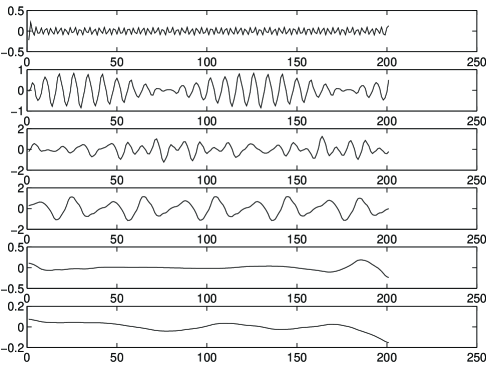
Figure 2: Contributions to approximation: from scale $2^{1}$ to $2^{5}$ (without noise).

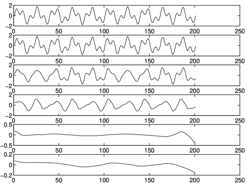
Figure 3: Approximations: from scale $2^{1}$ to $2^{5}$ (without noise).

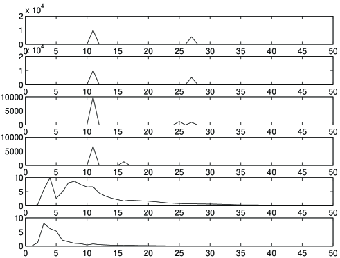
Figure 4: Power spectral density: from scale $2^{1}$ to $2^{5}$ (without noise)

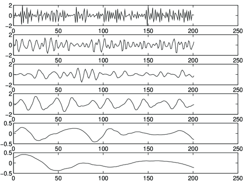
Figure 5: Contributions to approximation: from scale $2^{1}$ to $2^{5}$ (with noise).

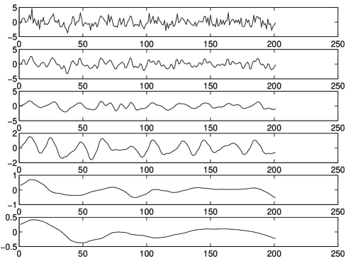
Figure 6: Approximations: from scale $2^{1}$ to $2^{5}$ (with noise).

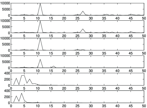
Figure 7: Power spectral density: from scale $2^{1}$ to $2^{5}$ (with noise)

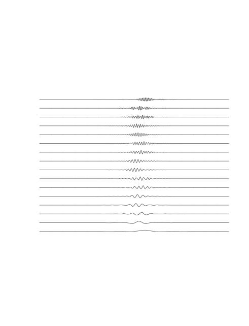
Figure 8: Localized contributions to beam motion.

References

- [1] J.B. Rosenzweig, Fundamentals of Beam Physics, e-version: http://www.physics.ucla.edu/class/99F/250_Rosenzweig/notes/
- [2] L. Serafini and J.B. Rosenzweig, Phys. Rev. E 55, 7565, 1997.
- [3] J.B. Rosenzweig, S.Anderson and L. Serafini, ‘Space Charge Dominated Envelope Dynamics of Asymmetric Beams in RF Photoinjectors’, Proc. PAC97 (IEEE,1998).
- [4] A.N. Fedorova and M.G. Zeitlin, ’Wavelets in Optimization and Approximations’, Math. and Comp. in Simulation, 46, 527, 1998.
- [5] A.N. Fedorova and M.G. Zeitlin, ’Wavelet Approach to Polynomial Mechanical Problems’, New Applications of Nonlinear and Chaotic Dynamics in Mechanics, 101 (Kluwer, 1998).
- [6] A.N. Fedorova and M.G. Zeitlin, ’Wavelet Approach to Mechanical Problems. Symplectic Group, Symplectic Topology and Symplectic Scales’, New Applications of Nonlinear and Chaotic Dynamics in Mechanics, 31 (Kluwer, 1998).
-
[7]
A.N. Fedorova and M.G. Zeitlin,
’Nonlinear Dynamics of Accelerator via Wavelet
Approach’, CP405, 87 (American Institute of Physics, 1997).
Los Alamos preprint, physics/9710035. - [8] A.N. Fedorova, M.G. Zeitlin and Z. Parsa, ’Wavelet Approach to Accelerator Problems’, parts 1-3, Proc. PAC97 2, 1502, 1505, 1508 (IEEE, 1998).
- [9] A.N. Fedorova, M.G. Zeitlin and Z. Parsa, ’Nonlinear Effects in Accelerator Physics: from Scale to Scale via Wavelets’, ’Wavelet Approach to Hamiltonian, Chaotic and Quantum Calculations in Accelerator Physics’, Proc. EPAC98, 930, 933 (Institute of Physics, 1998).
-
[10]
A.N. Fedorova, M.G. Zeitlin and Z. Parsa,
Variational Approach in
Wavelet Framework to Polynomial
Approximations of Nonlinear Accelerator Problems.
CP468, 48 ( American Institute of Physics, 1999).
Los Alamos preprint, physics/990262 -
[11]
A.N. Fedorova, M.G. Zeitlin and Z. Parsa,
Symmetry, Hamiltonian
Problems and Wavelets in
Accelerator Physics.
CP468, 69 (American Institute of Physics, 1999).
Los Alamos preprint, physics/990263 -
[12]
A.N. Fedorova and M.G. Zeitlin,
Nonlinear Accelerator Problems
via Wavelets, parts 1-8,
Proc. PAC99,
1614, 1617, 1620, 2900, 2903,
2906, 2909, 2912 (IEEE/APS, New York, 1999).
Los Alamos preprints: physics/9904039, physics/9904040, physics/9904041, physics/9904042, physics/9904043, physics/9904045, physics/9904046, physics/9904047. - [13] A.N. Fedorova and M.G. Zeitlin, in press.
- [14] A. Latto, H.L. Resnikoff and E. Tenenbaum, Aware Technical Report AD910708, 1991.
- [15] G. Schlossnagle, J.M. Restrepo and G.K. Leaf, Technical Report ANL-93/34.
- [16] A. Cohen, I. Daubechies and J.C. Feauveau, Comm. Pure. Appl. Math., XLV, 485 (1992).
- [17] W. Dahmen, C. Micchelli, SIAM J. Numer. Anal., 30, 507 (1993).