Generalized Optimal Current Patterns and Electrical Safety in EIT

Abstract

There are a number of constraints which limit the current and voltages which can be applied on a multiple drive electrical imaging system. One obvious constraint is to limit the maximum Ohmic power dissipated in the body. Current patterns optimising distinguishability with respect to this constraint are singular functions of the difference of transconductance matrices with respect to the power norm. (the optimal currents of Isaacson). If one constrains the total current ($L^{1}$ norm) the optimal patterns are pair drives. On the other hand if one constrains the maximum current on each drive electrode (an $L^{\infty}$ norm), the optimal patterns have each drive channel set to the maximum source or sink current value. In this paper we consider appropriate safety constraints and discuss how to find the optimal current patterns with those constraints.

1 Introduction

The problem of optimizing the drive patterns in EIT was first considered by Seagar [1] who calculated the optimal placing of a pair of point drive electrodes on a disk to maximize the voltage differences between the measurement of a homogeneous background and an offset circular anomaly. Isaacson [2], and Gisser, Isaacson and Newell [3] argued that one should maximize the $L^{2}$ norm of the voltage difference between the measured and calculated voltages constraining the $L^{2}$ norm of the current patterns in a multiple drive system. Later [4] they used a constraint on the maximum dissipated power in the test object. Eyöboǧlu and Pilkington [7] argued that medical safety legislation demanded that one restrict the maximum total current entering the body, and if this constraint was used the distinguishability is maximized by pair drives. Cheney and Isaacson [5] study a concentric anomaly in a disk, using the ’gap’ model for electrodes. They compare trigonometric, Walsh, and opposite and adjacent pair drives for this case giving the dissipated power as well as the $L^{2}$ and power distinguishabilies. Köksal and Eyöboǧlu [6] investigate the concentric and offset anomaly in a disk using continuum currents.

Yet another approach [8] is to find a current pattern maximizing the voltage difference for a single differential voltage measurement.

2 Medical Electrical Safety Regulations

We will review the current safety regulations here, but notice that they were not designed with multiple drive EIT systems in mind and we hope to stimulate a debate about what would be appropriate safety standards.

For the purposes of this discussion the equipment current (“Earth Leakage Current” and “Enclosure Leakage Current”) will be ignored as the emphasis is on the patient currents. These will be assessed with the assumption that the equipment has been designed such that the applied parts, that is the electronic circuits and connections which are attached to the patient for the delivery of current and the measurement of voltage, are fully isolated from the protective earth (at least $50M\Omega$).

IEC601 and the equivalent BS5724 specify a safe limit of 100 $\mu$A for current flow to protective earth (“Patient Leakage Current”) through electrodes attached to the skin surface (Type BF) of patients under normal conditions. This is designed to ensure that the equipment will not put the patient at risk even when malfunctioning. The standards also specify that the equipment should allow a return path to protective earth for less than 5 mA if some other equipment attached to the patient malfunctions and applies full mains voltage to the patient. Lower limits of 10 $\mu$A (normal) and 50 $\mu$A (mains applied to the patient) are set for internal connections, particularly to the heart (Type CF), but that is not at present an issue for EIT researchers.

The currents used in EIT flow between electrodes and are described in the standards as “Patient Auxiliary Currents” (PAC). The limit for any PAC is a function of frequency, 100 microamps from 0.1Hz to 1 kHz; then $100f$ $\mu$A from 1 kHz to 100 kHz where $f$ is the frequency in kHz; then 10 mA above 100 kHz. The testing conditions for PAC cover 4 configurations; the worst case of each should be examined.

1. Normal conditions. The design of single or multiple current source tomographs should ensure that each current source is unable to apply more than the maximum values given.

2. The PAC should be measured between any single connection and all the other connections tied together. a) if the tomograph uses a single current source then the situation is similar to normal conditions (above) b) if the tomograph uses multiple current sources then as far as the patient is concerned the situation is the same as normal conditions. The design of the sources should be such that they will not be harmed by this test.

3. The PAC should be measured when one or more electrodes are disconnected from the patient. This raises issues for multiple-source tomographs : a) if an isolated-earth electrode is used then the current in it will be the sum of the currents which should have flowed in the disconnected electrodes; they could all be of the same polarity. The isolated-earth electrode should therefore include an over-current sensing circuit which will turn down/off all the current sources. b) If no isolated-earth electrode is used then the situation is similar to normal conditions.

4. The PAC should be measured when the disconnected electrodes are connected to protective earth. This introduces no new constraints given the tomograph is fully isolated.

3 Constrained Optimization

Let $V=(V_{1},\dots,V_{K})^{T}$ be the vector of potentials measured on electrodes when a pattern of currents $I=(I_{1},\dots,I_{K})^{T}$ is applied. These are related linearly by $R$ the transfer impedance matrix: $V=RI$. For simplicity we will assume the same system of electrodes is used for current injection and voltage measurement. We will also assume that the conductivity is real and the currents in-phase to simplify the exposition. A model of the body is used with our present best estimate for the conductivity and from this we calculate voltages $V_{\mathrm{c}}$ for the same current pattern. Our aim is to maximize the distinguishability $\|V-V_{\mathrm{c}}\|_{2}=\|(R-R_{\mathrm{c}})I\|_{2}$. The use of the $L^{2}$ norm here corresponds to the assumption that the noise on each measurement channel is independent and identically distributed. If there were no constraints on the currents the distinguishability would be unbounded.

The simplest idea [3] is to maximize $\|(R-R_{\mathrm{c}})I\|_{2}$ subject to $\|I\|_{2}\leq M$ for some fixed value of $M$. The solution of this problem that $I$ is the eigenvector of $R-R_{\mathrm{c}}$ corresponding to the largest (in absolute value) eigenvalue. One problem is that the 2-norm of the current has no particular physical meaning. In a later paper [4] it was proposed that the dissipated power be constrained, that is $I\cdot V=I^{T}RI$. The optimal current is the eigenvector of $(R-R_{\mathrm{c}})R^{-1/2}$. (The inverse implied in the expression $R^{-1/2}$ has to be understood in the generalized sense, that is one projects on to the space orthogonal to $(1,\dots,1)^{T}$ and then calculates the matrix exponent $1/2$.) In practical situations in medical EIT the total dissipated power is unlikely to be an active constraint, although local heating effects in areas of high current density may be an issue. Even in industrial applications of EIT, the limitations of voltages and currents handled by normal electronic devices mean that one is unlikely to see total power as a constraint. One exception might be in EIT applied to very small objects.

As we have seen a reasonable interpretation of the safety regulations is to limit the current on each electrode to some safe level $I_{\mathrm{max}}$. We will refer to this as an $L^{\infty}$ constraint. This corresponds to a convex system of linear constraints $-I_{\mathrm{max}}\leq I_{k}\leq I_{\mathrm{max}}$. When we maximize the square of the distinguishabilty, which is a positive definite quadratic function of $I$, with respect to this set of constraints it can be seen that the maximum must be a vertex of the convex polytope $\{I:\max_{k}\{|I_{k}|\}=I_{\mathrm{max}},\sum_{k}I_{k}=0\}$. For example, for an even number $2n$ of electrodes the ${}^{2n}C_{n}$ vertices are the currents with each $I_{k}=\pm I_{\mathrm{max}}$, and an equal number with each sign. For the circularly symmetric case these are the Walsh patterns referred to in  [5].

If one wanted to be safe under the multiple fault condition that all the electrodes driving a current with the same sign became disconnected, and the safety mechanism on the isolated-earth failed, one would employ the $L^{1}$ constraint $\sum_{k}|I_{k}|\leq 2I_{\mathrm{max}}$. Again this gives a convex feasible set. In this case a polyhedron with vertices $I$ such that all but two $I_{k}$ are zero, and those two are $I_{\mathrm{max}}$ and $-I_{\mathrm{max}}$. These are the pair drives as considered by Seagar. Pair drives were also considered by [5],[7],[6] for single circular anomalies. Notice that $L^{1}$ optimal currents will be pair drives for any two- or three-dimensional geometry and any conductivity distribution.

Another constraint which may be important in practice is that the current sources are only able to deliver a certain maximum voltage $V_{\mathrm{max}}$ close to their power supply voltage. If the EIT system is connected to a body with transfer impedance within its design specification then the constraints $-V_{\mathrm{max}}\leq V_{k}\leq V_{\mathrm{max}}$ will not be active. If they do become active then the additional linear constraints in $I$ space $-V_{\mathrm{max}}\leq R^{-1}I\leq V_{\mathrm{max}}$ (here $R^{-1}$ is to be interpreted as the generalized inverse), will still result in a convex feasible region.

When any of the linear constraints are combined with quadratic constraints such as maximum power dissipation the feasible set of currents is still convex but its surface is no longer a polytope.

4 Numerical Results

Although we can easily find the vertices of the feasible region there are too many for it to be wise to search exhaustively for a maximum of the distinguishability. For $32$ electrodes for example there are ${}^{32}C_{16}>6\times 10^{8}$. Instead we use a discrete steepest ascent search method of the feasible vertices. That is from a given vertex we calculate the objective function for all vertices obtained by changing a pair of signs, and move to whichever vertex has the greatest value of the objective function. For comparison we also calculated the $L^{2}$ optimal currents, the optimal currents for the power constraint, and the optimal pair drive ($L^{1}$ optimal).

We used a circular disk for the forward problem, and the EIDORS Matlab toolbox [9] for mesh generation and forward solution. The mesh and conductivity targets can be seen in Figure 3. Our results are interesting in that for the cases we have studied so far the $L^{\infty}$ optimal currents have only two sign changes. The distinguishabilies given in Table 1 should be read with caution, as it is somewhat unfair to compare for example power constrained with $L^{\infty}$ patterns. They are designed to optimise different criteria. However the contrast between pair drive and $L^{\infty}$ is worth noting as the majority of existing EIT systems can only drive pairs of electrodes.

The greatest current densities occur at the contact points between the electrode boundaries and skin. At each electrode this current density is determined mainly by the total electrode current, the contact impedance and the skin conductivity just below the electrode. These factors dominate the current density near the electrode boundaries and the other electrode’s currents have a much smaller contribution to the maximum current densities

5 Conclusions

If using optimal current patterns one should be sure to use the right constraints. We suggest that in many situations the $L^{\infty}$ constraint may be the correct one. We have demonstrated that it is simple to compute these optimal patterns, and the instrumentation required to apply these patterns is much simpler than the $L^{2}$ or power norm patterns. While still requiring multiple current sources, they need only be able to switch between sinking and sourcing the same current.

	Single anomaly		Two anomalies
Constraint	Voltage diff.	Power	Voltage diff.	Power
$L^{1}$ Best pair drive	440.0911	1200.7618	347.3579	1185.4935
$L^{2}$ optimal	812.3243	3356.3035	571.9161	3170.0985
Power optimal	518.9126	1768.3048	321.616	1352.6896
$L^{\infty}$ optimal	1653.2673	19261.9208	968.2656	16798.3363

Table 1: $L^{2}$ norm of voltage difference, and dissipated power for one and two anomalies with a variety of constraints. The constraint levels have been chosen so that the maximum electrode current is the same on each

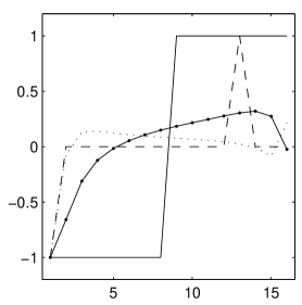
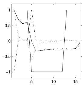
Figure 1: Optimal current patterns. Continuous line is the $L^{\infty}$ norm, $-\circ-$ is the $L^{2}$ optimal, $\cdots$ power norm optimal and $--$ is $L^{1}$ optimal (pair drive).

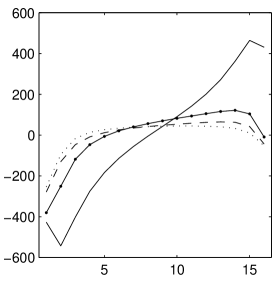
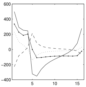
Figure 2: Voltage difference measurements for one and two anomalies. For key see figure 1

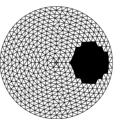
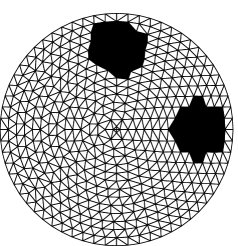
Figure 3: Mesh and conductivity anomalies.

References

- [1] A.D. Seagar, Probing with low frequency electric current, PhD Thesis, University of Canterbury, Christchurch, NZ, 1983.
- [2] D. Isaacson, Distinguishability of conductivities by electric-current computed-tomography, IEEE Trans. Med. Imaging 5, pp.91-95, 1986
- [3] G. Gisser, D. Isaacson and J.C. Newell, Current topics in impedance imaging, Clin. Phys. Physiol. Meas., 8 Suppl A, pp39–46, 1987.
- [4] G. Gisser, D. Isaacson and J.C. Newell, Electric Current computed-tomography and eigenvalues, SIAM J. Appl. Math., 50 pp.1623-1634, 1990.
- [5] M. Cheney, and D. Isaacson, Distinguishability in Impedance Imaging, IEEE Trans. Biomed. Eng., 39, pp. 852-860, 1992.
- [6] A. Köksal and B. M. Eyüboǧlu Determination of optimum injected current patterns in electrical impedance tomography, Pysiol Meas 16, ppA99-A109, 1995.
- [7] B.M. Eyüboǧlu and T.C. Pilkington Comment on Distinguishability in Electrical-Impedance Imaging, IEEE Trans. Biomed. Eng.,40, pp.1328-1330,1993
- [8] Breckon W.R., Measurement and reconstruction in electrical impedance tomography, in ‘Inverse problems and imaging’, Ed. G.F. Roach, Pitman Res. Notes in Math., 245 , pp1-19, 1991.
- [9] Vauhkonen M. et al, A Matlab Toolbox for the EIDORS project to reconstruct two- and three-dimensional EIT images, Pysiol. Meas. to appear.