Interfering with Interference: a Pancharatnam Phase Polarimeter

Abstract

A simple variation of the traditional Young’s double slit experiment can demonstrate several subtleties of interference with polarized light, including Berry and Pancharatnam’s phase. Since the position of the fringes depends on the polarization state of the light at the input, the apparatus can also be used to measure the light’s polarization without a quarter-wave plate or an accurate measurement of the light’s intensity. In principle this technique can be used for any wavelength of photon as long as one can effectively polarize the incoming radiation.

I Introduction

Pancharatnam [1] explored how the phase of polarized light changes as the light passes through cycle of polarizations. He found that the phase increases by $-\Omega/2$, where $\Omega$ is the solid angle that the geodesic path of polarizations subtends on the Poincaré sphere. If the path does not consist of great circles, an additional dynamical phase will develop. Berry [2] developed corresponding theory for general quantum systems and re-derived Pancharatnam’s result [3].

A series of experiments have been performed which demonstrate the Pancharatnam phase [4, 5, 6, 7, 8, 9, 10, 11] and the related geometric phase [12, 13, 14]. De Vito and Levrero [15] have criticized many of these experiments because they use retarders which introduce a dynamical component to the phase. Berry & Klein [16] and Hariharan et al. [17, 18] have performed a series of experiments using only polarizers and beam splitters to introduce and measure the geometric phase.

In this paper, I describe a simple experiment using polarizers and a double slit to demonstrate the Pancharatnam phase and use this phase to determine the polarization state of the incoming light. If the incoming light is linearly polarized and the polarizers are also linear, the resulting phase is limited to 0 or $\pi$. However, elliptically polarized light will result in intermediate values of the phase. This experiment uses a double slit rather than a half silvered mirror to split the beam, eliminating a possible source of dynamic phase; furthermore, with fewer and less complex optical elements this experiment may be performed over a wide range of photon energies. Furthermore, since the optics are simple, one can analyze the experiment in terms of Maxwell’s equations, illustrating the connection between these equations and the Pancharatnam phase.

II Experimental Apparatus

Fig. 1 illustrates the experiment setup (c.f. [19, 20, 21]). RP and FP denote rotatable and fixed linear polarizers respectively. Each fixed linear polarizer covers one of the two slits and is oriented perpendicular to the other. Each rotatable polarizer is oriented at forty-five degrees to the polarizers to maximize throughput. Incidentally, if the final polarizer is removed, the interference pattern disappears according to the Frensel-Arago law [19].

The arrangement is similar to that used by Schmitzer, Klein & Dultz [11]. Instead of using a Babinet-Soleil compensator to vary the geometric phase. The phase depends on the input and output polarizations of interferometer. If the two polarizers are aligned, the Pancharatnam phase between the two paths vanishes; and if they are orthogonal, the phase is $\pi$.

FIG. 1.: Optical system of the Pancharatnam phase polarimeter

The setup is identical to the standard physics demonstration of Young’s double-slit experiment with the exception that each slit is covered with a polarizing filter; consequently, both the construction and analysis of the experiment are amenable as a demonstration or student laboratory experiment. Furthermore, the light follows the same spatial trajectory, independent of the position of the polarizers and the geometric phase observed.

III The Poincaré Sphere

Understanding how the apparatus works for a general polarization is most simply achieved by tracing the polarization of the light through the system along the Poincaré sphere. The initial polarization from the laser is unknown but it is depicted in the figures as left circular. The left panel of Fig. 2 depicts the configuration for zero geometric phase. As the laser passes through the first polarizer, its polarization is projected onto the horizontal direction. After passing through the two slits, the polarization is projected onto two orthogonal polarizations oriented at forty-five degrees to the horizontal. Finally, the last polarizer projects the polarization back onto the horizontal. One can form a closed loop by following the path along one leg and returning along the other leg (c.f.  [11]). This closed loop does not enclose any solid angle on the sphere.

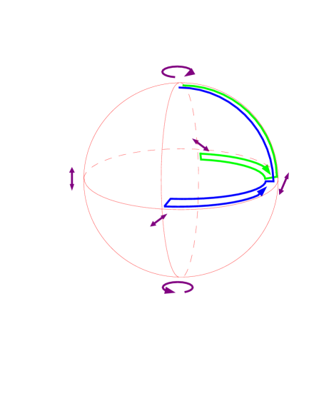
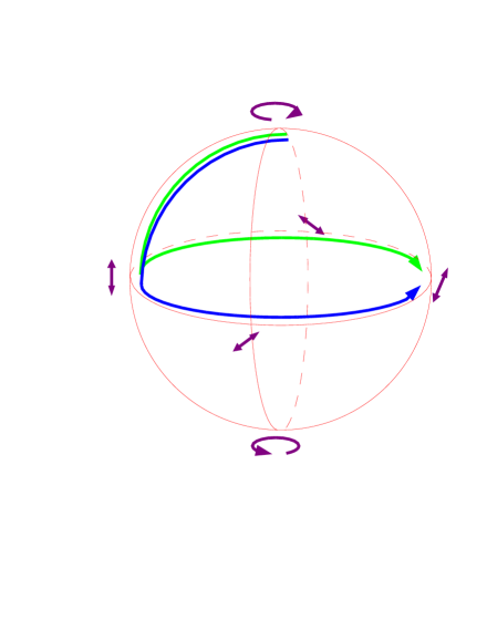
FIG. 2.: The path the polarization follows on the Poincaré sphere for the input and output polarizers aligned in parallel (left) and orthogonally (right).

The right panel of Fig. 2 illustrates the path of the polarization when the two rotatable polarizers are orthogonal. The polarization is now projected onto the vertical first, followed by the two diagonal polarizations and the final horizontal projection. Constructing the closed loop as described earlier yields an area of $2\pi$ and a Pancharatnam phase of $-\pi$ between the two slits.

Since a constant phase difference of $\pi$ is equivalent to $-\pi$, this implementation hides the fact that the area on the sphere is oriented and consequently the geometric phase may be positive or negative. A third configuration when the input polarizer is followed by a quarter-wave plate yielding right-hand circular polarized input to the interferometer illustrates this point. The direction that the loop is traversed determines which slit is designated by $\phi_{1}$ such that $\phi_{1}-\phi_{2}=-\Omega/2$. The phase difference is given by $\pi/2$ if the final polarizer lies clockwise relative to polarizer behind the first slit, and $-\pi/2$ if the final polarizer lies counterclockwise. The converse result holds for left-hand polarized light.

If the axis of polarizer behind left-hand slit (as one looks toward the screen) lies clockwise of that of the final polarizer, one obtains the result that the fringes will shift to the left (relative to their position for the input and output polarizations being identical) if the light is left elliptically polarized and to the right if it is right elliptically polarized. This configuration automatically includes the minus sign present in Pancharatnam’s definition of the geometric phase. The upper and lower panels of Fig. 3 show the fringe pattern produced by the apparatus in the configuration described above for the input and output polarizations being linear and identical and linear and orthogonal. The middle panel shows the fringes for left-hand circularly polarized input light at the input with the input polarizer removed.

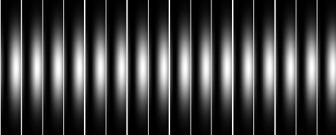
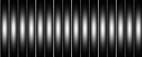
FIG. 3.: Schematic of the interference patterns for $\phi_{1}-\phi_{2}=0,\pi/2,\pi$ for quasi-monochromatic light.

IV Measuring the Input Polarization

If the input polarizer is removed, the apparatus can be used to measure the polarization of the light source. The procedure requires four measurements of the fringe positions: two for calibration and two to determine the geometric phases.

1. Locate the positions of the fringes with the input and output polarizers parallel and midway between the polarizers at the slits.

2. Remove the input polarizer and compare the position of the fringes relative to the two previous measurements. Let $\alpha/(2\pi)$ be the ratio of the offset of the fringes in step (2) relative to step (1) to the distance between the fringes in step (1). Also, note the direction that fringes shift – left for left-circular polarization and right for right-circular polarization.

3. Rotate either all of the polarizers by forty-five degrees or rotate the light source by forty-five degrees and repeat steps (1) and (2) and denote the resulting ratio by $\beta/(2\pi)$.

The left panel of Fig. 4 depicts how the polarization evolves on the Poincaré sphere for the two configurations. It is straightforward to calculate the input polarization using spherical trigonometry by following the right panel of Fig. 4. $\sin d$ gives the fraction of circular polarization and $e$ is the angle between the long axis of the polarization ellipse and the vertical axis. Napier’s analogies yield

$$a=-\left\{\tan^{-1}\left[\frac{\sin\frac{1}{2}(\alpha-\beta)}{\sin\frac{1}{2}(\alpha+\beta)}\right]+\tan^{-1}\left[\frac{\cos\frac{1}{2}(\alpha-\beta)}{\cos\frac{1}{2}(\alpha+\beta)}\right]\right\}$$ (1)

and the law of sines gives

$$\sin d=\sin a\sin\beta.$$ (2)

Combining these two results yields

$$\tan\frac{e}{2}=\tan\frac{1}{2}(a-d)\frac{\sin\left(\frac{\pi}{4}+\frac{\beta}{2}\right)}{\sin\left(\frac{\pi}{4}-\frac{\beta}{2}\right)}$$ (3)

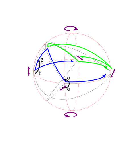
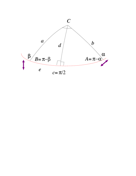
FIG. 4.: Measuring and calculating the input polarization

If the input polarization is linear, one finds that measurements of the fringes can only locate the polarization vector to within forty-five degrees. However, the contrast of the interference pattern constrains the linear polarization further, as well as the fractional polarization of the input light.

V Conclusions

A variation of Young’s double-slit experiment provides a excellent and simple demonstration of the Pancharatnam phase for polarized light. Furthermore, the observed phase difference between the two slits is simply related to the polarization of the incoming light. The phase difference determines upon which great circle of the Poincaré sphere the polarization lies, and by performing the measurement after rotating the apparatus the input polarization can be determined precisely.

The distinct advantage of the experiment is the simplicity of the optics. Only linear polarizers and a double slit are required. Since the Pancharatnam phase is achromatic, the procedure may be performed for the wide range of photon energies where suitable materials are available. A companion paper discusses the implementation of the experiment in X-rays and possible applications.

REFERENCES

- [1] S. Pancharatnam, Proc. Indian Acad. Sci 44, 247 (1956).
- [2] M. V. Berry, Proc. R. Soc. Lond. A 392, 84 (1984).
- [3] M. V. Berry, J. Mod. Opt. 34, 1401 (1987).
- [4] R. Bhandari, Phys. Lett. A. 133, 1 (1988).
- [5] R. Bhandari and J. Samuel, Phys. Rev. Lett. 60, 1211 (1988).
- [6] R. Simon, H. J. Kimble, and E. C. G. Sudarshan, Phys. Rev. Lett. 61, 19 (1988).
- [7] R. Bhandari and T. Dasgupta, Phys. Lett. A. 143, 170 (1990).
- [8] R. Bhandari, Phys. Lett. A. 171, 262 (1992).
- [9] R. Bhandari, Phys. Lett. A. 171, 267 (1992).
- [10] R. Bhandari, Phys. Lett. A. 180, 21 (1993).
- [11] H. Schmitzer, S. Klein, and W. Dultz, Phys. Rev. Lett. 71, 1530 (1993).
- [12] R. Y. Chiao and W. S. Wu, Phys. Rev. Lett. 57, 933 (1986).
- [13] A. Tomita and R. Y. Chiao, Phys. Rev. Lett. 57, 937 (1986).
- [14] R. Y. Chiao et al., Phys. Rev. Lett. 60, 1214 (1988).
- [15] E. De Vito and A. Levrero, J. Mod. Opt. 41, 2233 (1994).
- [16] M. V. Berry and S. Klein, J. Mod. Opt. 43, 165 (1996).
- [17] P. Hariharan, H. Ramachandran, K. A. Suresh, and J. Samuel, J. Mod. Opt. 44, 707 (1997).
- [18] P. Hariharan, S. Mujumdar, and H. Ramachandran, J. Mod. Opt. 46, 1443 (1999).
- [19] E. Fortin, Am. Jour. Phys. 38, 917 (1970).
- [20] J. L. Hunt and G. Karl, Am. Jour. Phys. 38, 1249 (1970).
- [21] D. Pescetti, Am. Jour. Phys. 40, 735 (1972).