Temporal correlations and neural spike train entropy

Abstract

Sampling considerations limit the experimental conditions under which information theoretic analyses of neurophysiological data yield reliable results. We develop a procedure for computing the full temporal entropy and information of ensembles of neural spike trains, which performs reliably for limited samples of data. This approach also yields insight upon the role of correlations between spikes in temporal coding mechanisms. The method, when applied to recordings from complex cells of the monkey primary visual cortex, results in lower RMS error information estimates in comparison to a ‘brute force’ approach. PACS numbers: 87.19.Nn,87.19.La,89.70.+c,07.05.Kf

Cells in the central nervous system communicate by means of stereotypical electrical pulses called action potentials, or spikes [1]. The Shannon information content of neural spike trains is fully described by the sequence of times of spike emission. In principle, the pattern of spike times provides a large capacity for conveying information beyond that due to the code commonly assumed by physiologists, the number of spikes fired [2]. Reliable quantification of this spike timing information is made difficult by undersampling problems that scale with the number of possible spike patterns, and thus up to exponentially with the precision of spike observation (see Fig. 1). While advances have been made in experimental preparations where extensive sampling may be undertaken [3, 4, 5, 6], our understanding of the temporal information properties of nerve cells from less accessible preparations such as the mammalian cerebral cortex is limited.

Any direct estimate of the complete spike train information is limited by sampling considerations to relatively small wordlengths, and therefore to the analysis of short time windows of data. However, it is possible to take advantage of this restriction itself to obtain estimators which have better sampling properties than a ‘brute force’ approach. In this Letter we present an approach based upon a Taylor series expansion of the entropy, to second order in the time window of observation [7]. The analytical expression so derived allows the ensemble spike train entropy to be computed from limited data samples, and relates the entropy and information to the instantaneous probability of spike occurrence and the temporal correlations between spikes. Comparison with other procedures such as the ‘brute force’ approach [4, 9] indicates that our analytical expression gives substantially better performance for data sizes of the order typically obtained from mammalian neurophysiology experiments, as well as providing insight into potential coding mechanisms.

Consider a time period of duration $T$, associated with a dynamic or static sensory stimulus, during which the activity of $C$ cells is observed. The neuronal population response to the stimulus is described by the collection of spike arrival times $\{t^{a}_{i}\}$, $t^{a}_{i}$ being the time of the $i$-th spike emitted by the $a$-th neuron. The spike time is observed with finite precision $\Delta t$, and this bin width is used to digitise the spike train (Fig. 1). For a given discretisation (temporal precision), the entropy of the spike train is a well defined quantity. The total entropy of the spike train ensemble is

$$H(\{t^{a}_{i}\})=-\sum_{\{t_{i}^{a}\}}\;P(\{t_{i}^{a}\})\log_{2}P(\{t_{i}^{a}\}),$$ (1)

where the summation is over all possible spike times within $T$ and over all possible total spike counts from the population of cells. This entropy quantifies the total variability of the spike train. Each different stimulus history (time course of characteristics within $T$) is denoted as $s$. The noise entropy, which quantifies the variability to repeated presentations of the same stimulus, is $H^{\rm noise}=\left<H(\{t_{i}^{a}\}|s)\right>_{s}$, where the angular brackets indicate the average over different stimuli, $\left<A(s)\right>_{s}\equiv\sum_{s\in\cal S}P(s)A(s)$. The mutual information that the responses convey about which stimulus history invoked the spike train is the difference between these two quantities.

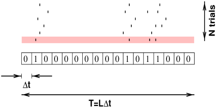
FIG. 1.: Digitising spike trains into binary ‘words’ with a given precision. A common experimental structure has $N$ repeats for each separate stimulus (one stimulus shown). The spike emission times for each such ‘trial’ are binned with resolution $\Delta t$, as shown for the last raster. There are $2^{L}$ possible words when examining data from a time window of duration $T$.

These entropies may be expanded as a Taylor series in the time window of measurement,

$$H=TH_{t}+\frac{T^{2}}{2}H_{tt}+O(T^{3}).$$ (2)

To compute the Taylor expansion, we made the following assumptions: (i) The time window is short enough, or the firing rate low enough, that there are few spikes per stimulus presentation. (ii) The entropy is analytic in $T$. (iii) Different trials are random realisations of the same process. We will use the bar notation for the average over trials at fixed stimulus, such that if $r_{a}(t;s)=\sum_{i}\delta_{t,t_{i}^{a}(s)}$, the time-dependent instantaneous firing rate $\overline{r}_{a}(t;s)$ is its average over experimental trials. (iv) Spikes are not locked to each other with infinite precision; in other words, the conditional probability of a spike occuring at time $\tau_{j}^{b}$ given occurrence of a particular spike pattern $\{t^{a}_{i}\}$ scales for small $\Delta t$ proportionally to $\Delta t$ plus higher order terms, with no $O(1)$ terms: $P(\tau_{j}^{b}|\{t^{a}_{i}\};s)\propto\Delta t+\cdots$ for each possible spike pattern $\{t^{a}_{i}\}$. The validity of these assumptions has been examined elsewhere [10].

The probability of observing a pattern with $k$ spikes can be expressed as a product of $k$ probabilities of each of the spikes given the presence of others. Thus from (iv), the probability of this pattern is proportional to $\Delta t^{k}$, and the expansion is essentially in the total number of spikes emitted. This also implies that only the conditional probabilities between spike pairs are necessary for the 2nd order expansion. Parameterising the conditional probability between two spikes by the scaled correlation $\gamma_{ab}(t^{a}_{i},t^{b}_{j};s)$ [11], we can now write down the probabilities required by Eq. 1.

Denoting the no spikes event as 0 and the joint occurrence of a spike from cell $a$ at time $t_{1}^{a}$ and a spike from cell $b$ at time $t_{2}^{b}$ as $t_{1}^{a}t_{2}^{b}$, the conditional response probabilities are, to second order:

$$P({\bf 0}|s) = 1-\;\sum_{a=1}^{C}\sum_{t_{1}^{a}}\overline{r}_{a}(t_{1}^{a};s)\Delta t+{1\over 2}\sum_{ab}\sum_{t_{1}^{a}}\sum_{t_{2}^{b}}\overline{r}_{a}(t_{1}^{a};s)\overline{r}_{b}(t_{2}^{b};s)\left[1+\gamma_{ab}(t_{1}^{a},t_{2}^{b};s)\right]\Delta t^{2}$$ (3)

$$P(t^{a}_{1}|s) = \overline{r}_{a}(t_{1}^{a};s)\Delta t-\overline{r}_{a}(t_{1}^{a};s)\sum_{b=1}^{C}\sum_{t_{2}^{b}}\overline{r}_{b}(t_{2}^{b};s)\left[1+\gamma_{ab}(t_{1}^{a},t_{2}^{b};s)\right]\Delta t^{2}\phantom{ppp}a=1,\cdots,C$$ (4)

$$P(t_{1}^{a}t_{2}^{b}|s) = \overline{r}_{a}(t_{1}^{a};s)\overline{r}_{b}(t_{2}^{b};s)\left[1+\gamma_{ab}(t_{1}^{a},t_{2}^{b};s)\right]\Delta t^{2}\phantom{ppp}a=1,\cdots,C,\qquad b=1,\cdots,C.$$ (5)

The unconditional response probabilities are simply $p(\{t_{i}^{a}\})=\left<p(\{t_{i}^{a}\}|s)\right>_{s}$. Inserting $p(\{t_{i}^{a}\})$ into Eq. 1 and keeping only leading order terms yields for the first order total entropy

$$TH_{t}=\frac{1}{\ln 2}\sum_{a}\sum_{t_{1}^{a}}\left<\overline{r}_{a}(t_{1}^{a};s)\Delta t\right>_{s}-\sum_{a}\sum_{t_{1}^{a}}\left<\overline{r}_{a}(t_{1}^{a};s)\Delta t\right>_{s}\log_{2}\left<\overline{r}_{a}(t_{1}^{a};s)\Delta t\right>_{s}.$$ (6)

Inserting $p(\{t_{i}^{a}\}|s)$ instead yields a similar expression for the first order noise entropy $TH^{\rm noise}_{t}$, except with a single stimulus average $\left<\cdot\right>_{s}$ around the entire second term. Continuing the expansion, and noting that a factor of 1/2 is introduced to prevent overcounting of equivalent permutations, the additional terms up to second order are:

$$\frac{T^{2}}{2}H_{tt} = \frac{1}{2\ln 2}\sum_{ab}\sum_{t_{1}^{a}}\sum_{t_{2}^{b}}\left\{\left<\overline{r}_{a}(t_{1}^{a};s)\overline{r}_{b}(t_{2}^{b};s)\left[1+\gamma_{ab}(t_{1}^{a},t_{2}^{b};s)\right]\right>_{s}-\left<\overline{r}_{a}(t_{1}^{a};s)\right>_{s}\left<\overline{r}_{b}(t_{2}^{b};s)\right>_{s}\right\}\Delta t^{2}$$ (8)

$$+\sum_{ab}\sum_{t_{t}^{a}}\sum_{t_{2}^{b}}\left<\overline{r}_{a}(t_{1}^{a};s)\overline{r}_{b}(t_{2}^{b};s)\left[1+\gamma_{ab}(t_{1}^{a},t_{2}^{b};s)\right]\Delta t^{2}\right>_{s}\log_{2}\frac{\left<\overline{r}_{a}(t_{1}^{a};s)\right>_{s}}{\sqrt{\left<\overline{r}_{a}(t_{1}^{a};s)\overline{r}_{b}(t_{2}^{b};s)\left[1+\gamma_{ab}(t_{1}^{a},t_{2}^{b};s)\right]\right>_{s}}}$$

$$\frac{T^{2}}{2}H_{tt}^{\rm noise} = \frac{1}{2\ln 2}\sum_{ab}\sum_{t_{1}^{a}}\sum_{t_{2}^{b}}\left<\overline{r}_{a}(t_{1}^{a};s)\overline{r}_{b}(t_{2}^{b};s)\gamma_{ab}(t_{1}^{a},t_{2}^{b};s)\right>_{s}\Delta t^{2}$$ (10)

$$+\sum_{ab}\sum_{t_{t}^{a}}\sum_{t_{2}^{b}}\left<\overline{r}_{a}(t_{1}^{a};s)\overline{r}_{b}(t_{2}^{b};s)\left[1+\gamma_{ab}(t_{1}^{a},t_{2}^{b};s)\right]\Delta t^{2}\log_{2}\frac{\overline{r}_{a}(t_{1}^{a};s)}{\sqrt{\overline{r}_{a}(t_{1}^{a};s)\overline{r}_{b}(t_{2}^{b};s)\left[1+\gamma_{ab}(t_{1}^{a},t_{2}^{b};s)\right]}}\right>_{s}.$$

The difference between the total and noise entropies gives the expression for the mutual information detailed in [10].

It has recently been found that correlations, even if independent of the stimulus identity, can increase the information present in a neural population [8, 12]. This applies both to cross-correlations between the spike trains from different neurons and to auto-correlations in the spike train from a single neuron [10]. The equations derived above add something to the explanation of this phenomenon provided in [8]. Observe that the second order total entropy can be rewritten in a form which shows that it depends only upon the grand mean firing rates across stimuli, and upon the correlation coefficient of the whole spike train, $\Gamma(t_{i}^{a},t_{j}^{b})$ (defined across all trials rather than those with a given stimulus as for $\gamma(t_{i}^{a},t_{j}^{b};s)$). Thus,

$$\frac{T^{2}}{2}H_{tt} = \frac{\Delta t^{2}}{2\ln 2}\sum_{ab}\sum_{t_{1}^{a}}\sum_{t_{2}^{b}}\left<\overline{r}_{a}(t_{1}^{a};s)\right>_{s}\left<\overline{r}_{b}(t_{2}^{b};s)\right>_{s}$$ (11)

$$\times \left\{\Gamma_{ab}(t^{a}_{i},t^{b}_{j})-[1+\Gamma_{ab}(t^{a}_{i},t^{b}_{j})]\ln[1+\Gamma_{ab}(t^{a}_{i},t^{b}_{j})]\right\}.$$ (12)

It follows that the second order entropy is maximal when $\Gamma=0$, and non-zero overall correlations in the spike trains (indicating statistical dependence) always decrease the total response entropy. $\gamma(s)$ acts on the noise entropy as $\Gamma$ does upon the total entropy – it can only decrease the conditional entropy. The effect of $\gamma(s)$ on the total entropy is more complex, depending upon the correlation of the firing across stimuli. $\gamma(s)$ can be chosen so as to increase the total entropy (and thus the information, with the noise entropy fixed), and this increase will be maximal for the $\gamma(s)$ which lead exactly to $\Gamma=0$. Neuronal or spike time interaction may therefore eliminate or reduce the effect of statistical dependencies introduced by other covariations.

The rate and correlation functions in practice must be estimated from a limited number of experimental trials, which leads to a bias in each of the entropy components. This bias was corrected for, as described in [13]; however, the sampling advantage that will be described was observed both with this correction, without bias correction, and with other bias correction approaches such as that used in [6].

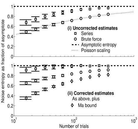
FIG. 2.: Data-size dependence of noise entropy estimates for a V1 complex cell. Time windows of 40ms (half a stimulus cycle) were broken into words of length 12 for the analysis. The upper panel, (i), shows entropy estimates prior to correction for bias, normalised by the asymptotic (true) entropy. The dotted line indicates the ‘brute force’ sampling characteristics for a Poisson process with the same time-dependent firing rate. The lower panel, (ii), shows the bias-corrected versions of these estimates, and in addition the Ma lower bound upon the entropy. The asymptotic entropy was obtained by extrapolating from the curves; the results agree to within 1%. Error bars were obtained by bootstrap resampling.

To demonstrate its applicability, we applied the series entropy analysis to data recorded from the primary visual cortex (V1) of anaesthetised macaque monkeys [15]. Fig. 2 examines, for a typical V1 complex cell, the dependence of the accuracy of the noise entropy estimate upon the number of experimental trials utilised. It is the noise entropy which is most affected by sampling constraints, so we shall concentrate upon this quantity here. The top panel shows the estimates before application of a bias removal procedure, using the series (our technique) and ‘brute force’ (simple application of Eqn. 1) approaches. The entropies are expressed as a fraction of the asymptotic entropy obtained by polynomial extrapolation [6]. Reliable extrapolation to the asymptotic entropy was possible because of the large amount of data that happened to be available for this cell (which was chosen with that in mind; more usually between 20 and 100 trials were available). This allowed us to compare the performance of the methods on smaller subsets of the data against a known reference. The fact that series and brute-force estimators converged for this cell indicates that higher order correlations amongst spike times contributed little to the entropy.

The better performance of the series approach can be understood by considering that (at second order) it requires sampling from only the first two moments of the probability distribution, whereas the ‘brute force’ approach depends upon all moments. Higher moments have to be computed from events with lower and lower probability, as shown in Eqn. 4; estimation of these lower probability events is more error-prone, and leads to the larger bias of the ‘brute force’ approach.

Also shown in Fig. 2 is the Ma lower bound upon the entropy [14], which has been proposed as a useful bound which is relatively insensitive to sampling problems [6]. The Ma bound is tight only when the probability distribution of words at fixed spike count is close to uniform. It can be seen that for the V1 complex cell data, the Ma bound is not tight at all. To understand the behaviour of the Ma bound for short time windows, we calculated series terms. The Ma entropy already differs from the true entropy at first order:

$$TH^{\rm Ma}_{t} = \frac{1}{\ln 2}\sum_{a}\sum_{t_{1}^{a}}\left<\overline{r}_{a}(t_{1}^{a};s)\Delta t\right>_{s}$$ (13)

$$- \sum_{a;t_{1}^{a}}\left<\overline{r}_{a}(t_{1}^{a};s)\Delta t\right>_{s}\log_{2}{\sum_{a;t_{1}^{a}}\left<\overline{r}_{a}(t_{1}^{a};s)\right>_{s}^{2}\Delta t\over\sum_{a;t_{1}^{a}}\left<\overline{r}_{a}(t_{1}^{a};s)\right>_{s}}$$ (14)

This coincides with Eqn. 5 only if there are no variations of rate across time and cells. If there were higher frequency rate variations, or more cells with different response profiles, the Ma bound would be still less useful.

Estimation quality depends upon not just sampling bias, but also variance; these can be summarised by the RMS error of the entropy estimate. We investigated the behaviour of the RMS error by fitting a Poisson model with matched time-dependent firing rate to the experimental data of Fig. 1. This model, although yielding a 5% lower noise entropy (because of correlations in the real data), predicted the ‘brute force’ sampling characteristics of Fig. 2 almost exactly. The model was used to generate a larger set of data (10,000 trials, or 160,000 stimulus presentations in total). This model yields worst-case sampling for the ‘brute force’ estimator; worst-case sampling for the series estimator would be achieved by even spread of probability throughout only the second order response space. The simulation serves to compare the estimators in a statistical regime similar to that of the typical cell of Fig. 2.

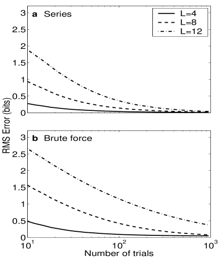
FIG. 3.: RMS error scaling characteristics for wordlengths from 4 to 12 in the simulation. The true noise entropies were 2.0, 3.5 and 4.7 bits respectively.

Fig. 3 shows the scaling of the RMS error before bias correction with data-size in this simulation. Scaling is qualitatively similar (but with a sharper decrease) after correction. The scaling behaviour resulting from the simulation predicts that with a ‘brute force’ approach, a RMS error of 2% of the entropy at a wordlength of 12 would require around 1400 trials with, and greater than 5000 trials without, application of the finite sampling correction. The series estimator reduces these requirements to approximately 50 and 400 trials respectively. These figures are dependent upon data statistics, and should be checked on a case by case basis; however, the dimensionality reduction with the series expansion provides a general improvement in the quality of entropy estimates for short time windows.

Some readers may wonder whether this new method amounts to computing the entropy with words with greater than 2 spikes thrown out. This is not the case: the proposed method considers pairwise interactions amongst all spikes in the word, no matter how many there are. It thus (unlike a truncated brute force approach) obtains the ability to take into account almost all of the entropy of longer words, while retaining the sampling benefits of being a second order method.

As neuroscience enters a quantitative phase, information theoretic techniques are being found useful for the analysis of data from physiological experiments. The methods developed here may broaden the scope of the study of neuronal information properties. In particular, they render feasible the information theoretic analysis of some recordings from anaesthetised and awake mammalian cerebral cortices.

SRS is supported by the HHMI, and SP by the Wellcome Trust.

REFERENCES

- [1] E. D. Adrian, J. Physiol. (Lond.) 61, 49 (1926).
- [2] D. MacKay and W. S. McCulloch, Bull. Math. Biophys. 14, 127 (1952).
- [3] F. Theunissen et al., J. Neurophys. 75, 1345, 1996; A. Dimitrov and J. P. Miller, Neurocomputing, 32-33, 1027, (2000).
- [4] R. R. de Ruyter van Steveninck et al., Science 275, 1805 (1997);
- [5] F. Rieke et al. Spikes: exploring the neural code (MIT Press, Cambridge, MA, USA, 1997).
- [6] S. Strong et al., Physical Review Letters 80, 197 (1998).
- [7] Previous studies have reported first order expansions of the information: W. E. Skaggs et al., in Adv. Neur. Inf. Proc. Sys., eds. S. Hanson, J. Cowan, and C. Giles (Morgan Kaufmann, San Mateo, 1993), Vol. 5, pp. 1030–1037; S. Panzeri et al., Network 7, 365 (1996).; N. Brenner et al. Neur. Comp. 12, 1531 (2000). Second order expansion of the spike count information from an ensemble of cells was performed in [8]. A cluster expansion method has also been used by M. DeWeese, Network 7, 325 (1996).
- [8] S. Panzeri et al. Proc. R. Soc. Lond. B 266, 1001 (1999).
- [9] G. T. Buracas et al., Neuron 20, 959 (1998).
- [10] S. Panzeri and S. R. Schultz, Neur. Comp. 13, in press.
-
[11]
The scaled correlation function is measured
as [8, 10]:
(15) (16) - [12] L.F. Abbott and P. Dayan, Neur. Comp. 11, 91-101 (1999); M. W. Oram et al., Trends in Neurosci. 21, 259-265 (1998).
- [13] S. Panzeri and A. Treves, Network 7, 87 (1996); M. S. Roulston, Physica D 125, 285 (1999).
- [14] S.-K. Ma, J. Stat. Phys. 26, 221 (1981).
- [15] The data used was from procedures to extract the direction tuning of V1 complex (non phase-modulated) cells. The stimuli were drifting sinusoidal gratings of 16 different directions placed over the receptive field of the cell. Periods of 40ms, or one half of the grating cycle, of both phases, were extracted for use as data trials. The cell used in Fig. 1, 470l006, was typical of the dataset. We thank J. R. Cavanaugh, W. Bair and J.A. Movshon, Soc. Neurosci. Abstr., 24, 1875 (1998), for making their data available to us.