Solitons in anharmonic chains
with ultra-long-range interatomic interactions

Abstract

We study the influence of long-range interatomic interactions on the properties of supersonic pulse solitons in anharmonic chains. We show that in the case of ultra-long-range (e.g., screened Coulomb) interactions three different types of pulse solitons coexist in a certain velocity interval: one type is unstable but the two others are stable. The high-energy stable soliton is broad and can be described in the quasicontinuum approximation. But the low-energy stable soliton consists of two components, short-range and long-range ones, and can be considered as a bound state of these components.

As is well known [1, 2], anharmonic chains with interactions between nearest neighbors can bear pulse solitons, compressive localized excitations which are very robust and propagate with supersonic velocities without energy loss. Because of their coherence, the solitons play an important role in determination of dynamical, thermodynamic, and transport properties of one-dimensional anharmonic systems [1]. Among other things, they have been invoked in order to explain energy transport in DNA [3].

However, the interatomic interactions in real systems are strictly speaking long-ranged. In particular, the DNA molecule contains charged groups with Coulomb interactions between them [4]. Therefore, it is essential to clarify how the long-range interactions (LRI’s) can affect the soliton features. It is generally believed that such interactions are very small (in comparison with the anharmonic interactions between nearest neighbors) and can be safely neglected. However, as we show in the present paper, even very weak LRI’s cause new qualitative effects if the interactions are ultra-long-ranged. A striking illustration is a chain with pure (not screened) Coulomb interactions between charged particles where the sound velocity is infinite regardless of the intensity of these interactions. As a consequence the pulse solitons merely do not exist in such a model (whereas the pure Coulomb interactions do not prevent [5] the existence of immobile intrinsic localized modes therein). Generally, arbitrary LRI’s introduce into the system a new length scale, the so-called radius of the LRI’s. If the radius of the LRI’s far exceeds the interatomic distance, the competition between the length scales manifests itself in a number of qualitative effects (see Refs. [6, 7] for the exponential-law LRI’s and Refs. [8, 9, 10] for the power-law LRI’s). The greater is the radius of the LRI’s, the more pronounced are these effects.

In this paper we show that two types of stable pulse solitons can coexist in a certain interval of velocities in anharmonic chains with ultra-long-range interatomic interactions even if they are very weak.

Let us consider a chain of equally spaced particles of unit mass whose displacements from equilibrium are $u_{n}(t)$ and the equilibrium spacings are unity. The Hamiltonian of the system is given by

$$H=\sum_{n}\biggl{\{}\frac{1}{2}\biggl{(}\frac{du_{n}}{dt}\biggr{)}^{2}+V(u_{n+1}-u_{n})$$ (1)

$$+\frac{1}{2}\sum_{m>n}J_{m,n}(u_{m}-u_{n})^{2}\biggr{\}}\;,$$ (2)

with the anharmonic interactions $V(w)=w^{2}/2-w^{3}/3$ between nearest neighbors and the harmonic LRI’s $J_{m,n}=J(e^{\alpha}-1)\,e^{-\alpha|m-n|}/|m-n|^{s}$ between all particles of the chain. Here $J$ characterizes the intensity of the LRI’s whereas $\alpha$ and $s$ determine their inverse radius. The parameters $\alpha$ and $s$ are introduced to cover different physical situations from the limit of nearest-neighbor interactions ($\alpha\gg 1$ or $s\gg 1$) to the limit of ultra-long-range interactions ($\alpha\ll 1$ and $s\leq 3$). The Hamiltonian (1) generates equations of motion of the form

$$\frac{d^{2}w_{n}}{dt^{2}} + 2F(w_{n})-F(w_{n+1})-F(w_{n-1})$$ (3)

$$+ \sum_{m\neq n}J_{m,n}(w_{n}-w_{m})=0\;,$$ (4)

where $w_{n}=u_{n+1}-u_{n}$ are relative displacements and $F(w)\equiv dV(w)/dw=w-w^{2}$ .

We assume in what follows that $\alpha\neq 0$ (the case $\alpha=0$ has already been considered in Ref. [9]); in doing so we studied most extensively two cases: the physically important screened Coulomb interactions ($s=3$) and the Kac-Baker LRI’s ($s=0$). However, in view of the fact (tested numerically) that all cases with $0\leq s\leq 3$ lead to qualitatively the same results but the case $s=0$ allows also analytical consideration, we discuss only the case $s=0$ from this point on.

In the quasicontinuum limit, treating $n$ as a continuous variable [$n\to x$ , $w_{n}(t)\to w(x,t)$, $w_{m}(t)\to e^{(m-n)\partial_{x}}w(x,t)$] and keeping formally all terms in the Taylor expansion of $e^{(m-n)\partial_{x}}$, the equation of motion (3) for $s=0$ can be cast in the operator form [7]

$$[\partial^{2}_{t}-JQ(\alpha,\partial_{x})]w(x,t)-4\sinh^{2}\biggl{(}\frac{\partial_{x}}{2}\biggr{)}F(w)=0\;,$$ (5)

where

$$Q(\alpha,\partial_{x})=(e^{\alpha}+1)\frac{4\sinh^{2}(\partial_{x}/2)}{\kappa^{2}-4\sinh^{2}(\partial_{x}/2)}$$ (6)

with $\kappa=2\sinh(\alpha/2)$ is a linear pseudo-differential operator. The speed of sound $c$ (which is an upper limit of the group velocity of linear waves), determined by the expression $c^{2}=1+J(1+e^{-\alpha})/(1-e^{-\alpha})^{2}$ , grows indefinitely as $\alpha$ decreases.

We are interested in the stationary soliton solutions $w(x,t)\equiv w(x-vt)$ propagating with velocity $v$. In this way we reduce our problem to a nonlinear eigenvalue problem with $v$ being a spectral parameter. Indeed, substituting $z=x-vt$ and using the continuum approximation $4\sinh^{2}(\partial_{x}/2)\approx\partial_{x}^{2}$, we can write Eq. (5) in the form [7]

$$(\partial_{z}^{2}-s_{+}^{2})(\partial_{z}^{2}-s_{-}^{2})w(z)=\frac{12}{v^{2}}(\partial_{z}^{2}-\kappa^{2})w^{2}(z)\;,$$ (7)

where the parameters $s_{\pm}$ are given by

$$s^{2}_{\pm}=\frac{1}{2} \bigg{\{}\kappa^{2}+12\frac{v^{2}-1}{v^{2}}$$ (8)

$$\pm \sqrt{\left(\kappa^{2}-12\frac{v^{2}-1}{v^{2}}\right)^{2}+48\kappa^{2}\frac{c^{2}-1}{v^{2}}}\bigg{\}}\;.$$ (9)

The parameter $s_{+}$ is finite at all velocities $v\geq c$ and tends to $\sqrt{12}$ for $v\to\infty$. The parameter $s_{-}$ vanishes at $v=c$ and tends to $\kappa$ for $v\to\infty$. Using the Green’s function method [9] one can show that stationary soliton solutions exist only for supersonic velocities $v>c$. The properties of these solitons are determined by the ratio of $s_{+}$ and $s_{-}$. In Fig. 1 we plot the energy of the soliton solutions of Eq. (5) which were found numerically using the method developed in Ref. [9].

The soliton energy grows monotonically with the velocity in the case of large $\alpha$ (see, e.g., $\alpha=0.3$ in Fig. 1). In this case the soliton properties are qualitatively the same as in the limit of nearest-neighbor interactions (NNI’s) for which Eq. (5) reduces to the Boussinesq equation. It is well known that this equation has a sech-shaped soliton solution $w(z)=-1.5\,(v^{2}-c^{2})/\cosh^{2}(\sigma z)$, where $\sigma=\sqrt{3(v^{2}-c^{2})}$ is the inverse soliton width. As indicated above, the energy $H\sim(v^{2}-c^{2})^{3/2}$ of these solitons is monotonic function of the velocity, which means that there is only one soliton state for each given value of energy or velocity.

FIG. 1.: Energy of the pulse solitons versus velocity found numerically for different values of $\alpha$ and $J$ (the value of $J$ was chosen to get constant $c=1.515$; see stars in Fig. 3): $\alpha=0.3$ and $J=0.05$ (dot-dashed line); $\alpha=0.17$ and $J=0.0172$ (long-dashed line); $\alpha=0.1$ and $J=0.0062$ (dashed line); $\alpha=0.05$ and $J=0.0016$ (full line).

FIG. 2.: Shapes of pulse solitons found numerically for different velocities at $\alpha=0.17$ and $J=0.0172$.

In the case of small $\alpha$ the soliton properties become much more interesting [6, 7]. As it was recently shown [7], two branches of stable supersonic pulse solitons should be distinguished in this case: low-velocity and high-velocity solitons, separated by a gap with unstable soliton states.

The solitons of the low-velocity branch are broad (they have a width much larger than $1/s_{+}$), and can be described by Eq. (7) in the approximation $(\partial_{z}^{2}-s_{+}^{2})w\approx-s_{+}^{2}w$. In this approximation the soliton solutions exist in a finite interval of velocities, $c<v<v_{cr}\simeq\sqrt{(4c^{2}-1)/3}$, and change their shape from the sech-form at $v\gtrsim c$ (see the case $v=1.6$ in Fig. 2) to the crest-form $w(z)\sim\exp(-\alpha|z|/2)$ for $v\to v_{cr}$ (see the case $v=1.652$ in Fig. 2). Such crest solitons (or peakons) were first introduced in the theory of shallow water motion [11, 12].

The solitons of the high-velocity branch are made up of two components: $w=w_{S}(z)+w_{L}(z)$, where the short-range component

$$w_{S}(z)\approx-\frac{s_{+}^{2}v^{2}}{8}(1-2\gamma)\,\mbox{sech}^{2}\biggl{(}\sqrt{1-2\gamma}\,\frac{s_{+}z}{2}\biggr{)}$$ (10)

is dominant in the center of the strain, while the long-range component $w_{L}(z)\simeq-\gamma\,(s_{+}^{2}v^{2}/12)\exp(-s_{-}|z|)$ is dominant in the tails (see the case $v=1.75$ in Fig. 2). It should be stressed that this division of the soliton body into two components is not just a mathematical trick. Our present numerical simulations testify that the solitons of the high-velocity branch can be considered as bound states of the short-range and long-range components: they can be excited such that the relative distance between the components oscillates. However, such internal soliton oscillations are highly damped and should not play an important part in the nonlinear dynamics of the system. The parameter $\gamma$ is determined by the equation

$$\gamma\sqrt{A\gamma^{2}-2(A+2)\gamma/3+1}=3(A-1)\frac{s_{-}}{s_{+}}\sqrt{1-2\gamma}\;$$ (11)

with $A=\kappa^{2}/s_{-}^{2}$. This equation, derived in Ref. [7], has been there analyzed for small values of $J$ and $\alpha$, for which it has a unique solution at all values of velocity $v$. It has been shown that the interplay of the components $w_{S}(z)$ and $w_{L}(z)$ results in this case into nonmonotonic dependence of soliton energy $H$ on the velocity (see, e.g., the case $\alpha=0.17$ in Fig. 1), so that there is an energy interval where three soliton states with different velocities exist for each given value of energy. As is shown in Ref. [7], the low- and high-velocity states (with $dH/dv>0$) are stable while the intermediate state (with $dH/dv<0$) is unstable.

FIG. 3.: Three regions of the system parameters with qualitatively different properties of the pulse solitons. Full lines represent Eqs. (12) and (13). The points, marked off as circles and diamonds, were calculated numerically. Stars mark the parameters used in Fig. 1.

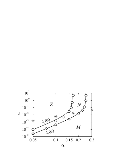
To sum up the foregoing, there is a demarcation line $J_{1}(\alpha)$ which separates the plane $\{\alpha,J\}$ into two regions (see Fig. 3), namely: the $M$-region (with a monotonic dependence of soliton energy on the velocity) at $J<J_{1}(\alpha)$ and the $N$-region (with a nonmonotonic dependence of soliton energy on the velocity) at $J>J_{1}(\alpha)$. Our numerical calculations (see Fig. 3) validate the following estimation for $J_{1}(\alpha)$:

$$J_{1}(\alpha)\simeq 0.23\,\frac{\alpha^{4}}{\alpha_{1}^{2}-\alpha^{2}}\;,$$ (12)

with $\alpha_{1}\simeq 0.25$. The spectrum of stable soliton states is continuous and covers all supersonic velocities in the $M$-region, while it has a gap (an interval of velocities with unstable soliton states) in the $N$-region. Emerging at $J=J_{1}(\alpha)$ this gap increases initially with growth of $J$. However, closer analytical examination of Eq. (11) shows that subsequently this gap starts to decrease and disappears again at $J=J_{2}(\alpha)>J_{1}(\alpha)$, where

$$J_{2}(\alpha)\simeq\frac{3}{8}\,\frac{\alpha^{4}}{\alpha_{2}^{2}-\alpha^{2}}\;,$$ (13)

with $\alpha_{2}\simeq 0.16$. Besides Eq. (13) we have found analytical expressions for the soliton energy and impulse, all in a very good agreement with the numerical calculations. But due to lack of place we do not present these cumbersome formulas in the present short paper. Instead, we just discuss below the results obtained for $J>J_{2}(\alpha)$ with the intent to demonstrate that the soliton features in this region (lets call it $Z$-region) are qualitatively different from those in the $N$-region.

FIG. 4.: Shapes of pulse solitons which coexist at the same velocity $v=1.64$, where $\alpha=0.05$ and $J=0.0016$. These solitons are also indicated on the inset of Fig. 1.

Indeed, when $J$ exceeds $J_{2}(\alpha)$ there appears an interval of velocities in which Eq. (11) has two real solutions. They correspond to two different types of two-component pulse solitons which coexist at the same velocity ($b$ and $c$ in Fig. 4). Accordingly, the dependence of the soliton energy on the velocity for $J>J_{2}(\alpha)$ is not merely nonmonotonic but takes on a $Z$-shaped multivalued form (see, e.g., the cases $\alpha=0.1$ and $\alpha=0.05$ in Fig. 1). The possibility of such a dependence has been predicted in Ref. [6] using a variational approach. At that time, however, this prediction was met with disbelief and considered as an artifact of variational approach. But as we prove numerically in the present paper, the $Z$-region really exists. In this region there is an interval of velocities where three soliton states of quite different shapes (see Fig. 4) and energies coexist at the same velocity. The soliton state with intermediate energy ($b$ in Fig. 4) is always unstable. But the high-energy and low-energy solitons ($a$ and $c$ in Fig. 4) are usually (when $dH/dv>0$) stable. The high-energy soliton on the low-velocity branch is broad and has a single component. But the low-energy soliton on the high-velocity branch and the soliton state with intermediate energy both consist of two components, short-range and long-range ones. The coexistence of two different types of stable pulse solitons at the same velocity causes new interesting phenomena, e.g., the synchronous propagation of two solitons with quite different widths (see Fig. 5).

FIG. 5.: Demonstration of the dynamical stability of the two stable pulse solitons ($a$ and $c$ in Fig. 4) which propagate with the same velocity $v=1.64$. Here $\alpha=0.05$ and $J=0.0016$.

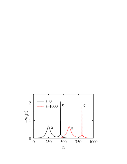
In conclusion, we show that the properties of pulse solitons in anharmonic chains with the long-range interatomic interactions are conveniently mapped onto the $\alpha J$-plane (see Fig. 3). One can recognize in this plane three regions with qualitatively different properties of the pulse solitons. The $M$- and $N$-regions were distinguished and discussed in Refs. [6, 7] whereas the $Z$-region (that is the region of ultra-long-range interatomic interactions) is proven to exist in the present paper. In this region there exists an interval of velocities where two types of stable pulse solitons coexist at each value of the velocity. The high-energy soliton is broad and has only a single component whereas the low-energy soliton consists of two components, short-range and long-range ones, and can be considered as a bound state of these components. It should be stressed that this phenomenon occurs even for LRI’s of very small intensity (hundreds times less than the intensity of NNI’s, as is seen on Fig. 3) if only the radius of LRI’s is large enough. It is important that the coexistence of two types of stable solitons does occur not only for the Kac-Baker LRI’s discussed in this paper; on the contrary, it is rather a common phenomenon. In particular, we also have shown that it exists in anharmonic chains with weakly screened Coulomb interactions between charged particles.

Two of us (Yu.G. and S.M.) thank the University of Bayreuth, where the main part of this work was done, for the hospitality. We also acknowledge the support provided by the DLR project UKR–002–99 of the scientific and technological cooperation between Germany and Ukraine.

REFERENCES

- [1] M. Toda, Theory of nonlinear lattices, Vol. 20 of Springer Series in Solid State Sciences, 2 ed. (Springer, Berlin, 1989).
- [2] N. Flytzanis, S. Pnevmatikos, and M. Remoissenet, J. Phys. C 18, 4603 (1985).
- [3] V. Muto, P. S. Lomdahl, and P. L. Christiansen, Phys. Rev. A 42, 7452 (1990).
- [4] S. F. Mingaleev, P. L. Christiansen, Yu. B. Gaididei, M. Johansson, and K. Ø. Rasmussen, J. Biol. Phys. 25, 41 (1999).
- [5] D. Bonart, Phys. Lett. A 231, 201 (1997); D. Bonart, T. Rössler, and J. B. Page, Physica D 113, 123 (1998).
- [6] A. Neuper, Yu. Gaididei, N. Flytzanis, and F. Mertens, Phys. Lett. A 190, 165 (1994).
- [7] Yu. Gaididei, N. Flytzanis, A. Neuper, and F. G. Mertens, Phys. Rev. Lett. 75, 2240 (1995); Physica D 107, 83 (1997).
- [8] Y. Ishimori, Prog. Theor. Phys. 68, 402 (1982).
- [9] S. F. Mingaleev, Yu. B. Gaididei, and F. G. Mertens, Phys. Rev. E 58, 3833 (1998).
- [10] S. Flach, Physica D 113, 184 (1998); Phys. Rev. E 58, R4116 (1998).
- [11] G. B. Whitham, Linear and nonlinear waves (Wiley, New York, 1974).
- [12] R. Camassa and D. D. Holm, Phys. Rev. Lett. 71, 1661 (1993).