Cross-Newell equations for hexagons and triangles

Abstract

The Cross-Newell equations for hexagons and triangles are derived for general real gradient systems, and are found to be in flux-divergence form. Specific examples of complex governing equations that give rise to hexagons and triangles and which have Lyapunov functionals are also considered, and explicit forms of the Cross-Newell equations are found in these cases. The general nongradient case is also discussed; in contrast with the gradient case, the equations are not flux-divergent. In all cases, the phase stability boundaries and modes of instability for general distorted hexagons and triangles can be recovered from the Cross-Newell equations.

1 Introduction

Hexagons are a very common planform arising in pattern-forming systems. The asymmetry between the centres and the edges of the hexagons leads to a favouring of hexagonal patterns in situations where there is intrinsic asymmetry, such as in Bénard-Marangoni convection [1]  [2] [3] where the top surface of the convecting layer is free and the bottom surface is in contact with a rigid boundary. Most natural systems will have some degree of asymmetry, and hence hexagons are widely observed, not only in convection experiments, but also for example in vibrated granular layers [4] [5] and during directional solidification [6]. Triangular patterns are more unusual, but are seen in some systems, such as vibrated granular layers [5].

Cross and Newell [7] pioneered a method of describing the behaviour of a fully nonlinear roll pattern in an extended system by following the evolution of the local phase, and hence the wavevector, associated with the roll pattern as it varies in space and time. This method was further developed by Passot and Newell [8] who regularised the Cross-Newell equations outside the region of roll stability, introducing an order parameter equation to account correctly for the behaviour of the pattern in regions where the amplitude is small.

The purpose of the current paper is to apply ideas similar to those of Cross & Newell [7] and Passot & Newell [8] to the evolution of fully nonlinear hexagonal and triangular patterns in large aspect ratio systems, such as those seen in experiments on Rayleigh-Bénard convection in $\rm SF_{6}$ near the thermodynamical critical point [9].

The paper is structured as follows: §2 presents a method of deriving the Cross-Newell equations for triangles and hexagons in a general real gradient system. The Cross-Newell equations for particular complex gradient systems are derived in §3 for hexagons and §4 for triangles. The case of free hexagons and triangles is discussed in §5, and the general nongradient case in §6. Section 7 concludes and indicates some directions for future investigation.

2 Derivation of the Cross-Newell equations

It is assumed that fully developed hexagons or triangles can be described by a stationary solution $w=w_{0}({\bf x})$ of an equation $w_{t}={\cal L}w+{\cal N}w$, where ${\cal L}$ and ${\cal N}$ are linear and nonlinear operators respectively, at least one of which is differential, with variational structure such that

$$\int dxdyw_{t}=-\int dxdy{\delta G\over\delta w},$$ (1)

where $w$ and $G(w)$ are real.

Hexagons and triangles are described by three wavevectors ${\bf k_{1}}$, ${\bf k_{2}}$ and ${\bf k_{3}}$ forming a resonant triad such that ${\bf k_{1}}+{\bf k_{2}}+{\bf k_{3}}={\bf 0}$. In the case where the governing equations force this resonance to be maintained, the pattern can be described using two phases $\theta_{1}$ and $\theta_{2}$ associated with two of these wavevectors ${\bf k_{1}}=\nabla\theta_{1}$ and ${\bf k_{2}}=\nabla\theta_{2}$. For fully nonlinear triangles and hexagons, the hexagon amplitude and the total hexagon phase $a=\theta_{1}+\theta_{2}+\theta_{3}$ (where ${\bf k_{3}}=-{\bf k_{1}}-{\bf k_{2}}=\nabla\theta_{3}$) are determined adiabatically from the two phases $\theta_{1}$ and $\theta_{2}$ except in the vicinity of defects where the amplitude is small or when the driving stress parameter of the system is close to the critical value for pattern formation so that the amplitude is small everywhere. In the ‘free’ case discussed in §5, where the resonant triad may be broken, the hexagon amplitude is slaved to the three independent phases $\theta_{1}$, $\theta_{2}$ and $\theta_{3}$, except when the amplitude is small.

In a large aspect ratio system, the size and orientation of the hexagons will typically change slowly in space and time. To describe these changes, it is convenient to introduce large scale phases $\Theta_{1}=\epsilon\theta_{1}$, $\Theta_{2}=\epsilon\theta_{2}$, where $\epsilon\ll 1$ is the inverse aspect ratio of the box, and slow space and time scales ${\bf X}=\epsilon{\bf x}$, $T=\epsilon^{2}t$. The local wavevectors are then given by ${\bf k_{i}}=\nabla_{\bf x}\theta_{i}=\nabla_{\bf X}\Theta_{i}$, $i=1,2$.

The hexagon solution is now considered to be a function of the two phases $\theta_{1}$ and $\theta_{2}$ and the slow space and time scales, such that $w\equiv w(\theta_{1},\theta_{2};{\bf X},T)$. Hence the space and time derivatives of $w$ are given by

$$\nabla_{\bf x}w(\theta_{1},\theta_{2};{\bf X},T) = ({\bf k_{1}}\partial_{\theta 1}+{\bf k_{2}}\partial_{\theta 2}+\epsilon\nabla_{\bf X})w(\theta_{1},\theta_{2};{\bf X},T),$$ (2)

$$\partial_{t}w(\theta_{1},\theta_{2};{\bf X},T) = (\epsilon\Theta_{1T}\partial_{\theta 1}+\epsilon\Theta_{2T}\partial_{\theta 2}+\epsilon^{2}\partial_{T})w(\theta_{1},\theta_{2};{\bf X},T).$$ (3)

To leading order then the following equations hold

$$w_{t} = \epsilon\{\Theta_{1T}(\partial_{\theta 1}w_{0})+\Theta_{2T}(\partial_{\theta 2}w_{0})\},$$ (4)

$$\delta w = (\partial_{\theta 1}w_{0})\delta\theta_{1}+(\partial_{\theta 2}w_{0})\delta\theta_{2}.$$ (5)

Substituting all this information into the governing equation ( 1) and averaging over $\theta_{1}$ and $\theta_{2}$ gives, to leading order in $\epsilon$,

$$\epsilon\int dxdy\overline{\{\Theta_{1T}(\partial_{\theta 1}w_{0})+\Theta_{2T}(\partial_{\theta 2}w_{0})\}\{(\partial_{\theta 1}w_{0})\delta\theta_{1}+(\partial_{\theta 2}w_{0})\delta\theta_{2}\}}$$

$$= -\int dxdy{\partial{\overline{G}}\over\partial k_{1}^{2}}\delta k_{1}^{2}+{\partial{\overline{G}}\over\partial k_{2}^{2}}\delta k_{2}^{2}+{\partial{\overline{G}}\over\partial{\bf(k_{1}.k_{2})}}\delta({\bf k_{1}.k_{2}}),$$ (6)

where $\overline{(.)}$ denotes the averaging. Remarking that $\delta k_{1}^{2}=\delta(\nabla_{\bf x}\theta_{1}.\nabla_{\bf x}\theta_{1})=2\nabla_{\bf x}\theta_{1}.\nabla_{\bf x}\delta\theta_{1}=2{\bf k_{1}}.\nabla_{\bf x}\delta\theta_{1}$, and similarly that $\delta k_{2}^{2}=2{\bf k_{2}}.\nabla_{\bf x}\delta\theta_{2}$ and $\delta({\bf k_{1}.k_{2}})={\bf k_{1}}.\nabla_{\bf x}\delta\theta_{2}+{\bf k_{2}}.\nabla_{\bf x}\delta\theta_{1}$, the divergence theorem can be used with suitable boundary conditions, to show that

$$\epsilon\int dxdy\overline{\{\Theta_{1T}(\partial_{\theta 1}w_{0})+\Theta_{2T}(\partial_{\theta 2}w_{0})\}\{(\partial_{\theta 1}w_{0})\delta\theta_{1}+(\partial_{\theta 2}w_{0})\delta\theta_{2}\}}$$

$$= \epsilon\int dxdy\nabla.\left\{2{\bf k_{1}}{\partial{\overline{G}}\over\partial k_{1}^{2}}\right\}\delta\theta_{1}+\nabla.\left\{2{\bf k_{2}}{\partial{\overline{G}}\over\partial k_{2}^{2}}\right\}\delta\theta_{2}$$ (7)

$$+\epsilon\int dxdy\nabla.\left\{({\bf k_{1}}\delta\theta_{2}+{\bf k_{2}}\delta\theta_{1}){\partial{\overline{G}}\over\partial{\bf(k_{1}.k_{2})}}\right\},$$

where $\nabla\equiv\nabla_{\bf X}=\epsilon^{-1}(\nabla_{\bf x}-{\bf k_{1}}\partial_{\theta 1}-{\bf k_{2}}\partial_{\theta 2})$. Since $\delta\theta_{1}$ and $\delta\theta_{2}$ are arbitrary, it is possible to extract the phase equations

$$\Theta_{1T}\overline{|\partial_{\theta 1}w_{0}|^{2}}+\Theta_{2T}\overline{(\partial_{\theta 1}w_{0})(\partial_{\theta 2}w_{0})} = \nabla.\left(2{\bf k_{1}}{\partial{\overline{G}}\over\partial k_{1}^{2}}+{\bf k_{2}}{\partial{\overline{G}}\over\partial{\bf(k_{1}.k_{2})}}\right),$$ (8)

$$\Theta_{2T}\overline{|\partial_{\theta 2}w_{0}|^{2}}+\Theta_{1T}\overline{(\partial_{\theta 1}w_{0})(\partial_{\theta 2}w_{0})} = \nabla.\left(2{\bf k_{2}}{\partial{\overline{G}}\over\partial k_{2}^{2}}+{\bf k_{1}}{\partial{\overline{G}}\over\partial{\bf(k_{1}.k_{2})}}\right).$$ (9)

The phase stability boundaries for general distorted hexagons and triangles defined by wavevectors ${\bf k_{1}}$ and ${\bf k_{2}}$ can be recovered from the Cross-Newell equations by first writing the equations explicitly in terms of the phases to give

$$\Theta_{1T}\overline{|\partial_{\theta 1}w_{0}|^{2}}+\Theta_{2T}\overline{(\partial_{\theta 1}w_{0})(\partial_{\theta 2}w_{0})}=$$

$$\nabla.\left\{2\nabla\Theta_{1}{\partial{\overline{G}}\over\partial k_{1}^{2}}(|\nabla\Theta_{1}|^{2},|\nabla\Theta_{2}|^{2},(\nabla\Theta_{1}.\nabla\Theta_{2}))\right\}+$$

$$\nabla.\left\{\nabla\Theta_{2}{\partial{\overline{G}}\over\partial{\bf(k_{1}.k_{2})}}(|\nabla\Theta_{1}|^{2},|\nabla\Theta_{2}|^{2},(\nabla\Theta_{1}.\nabla\Theta_{2}))\right\},$$ (10)

$$\Theta_{2T}\overline{|\partial_{\theta 2}w_{0}|^{2}}+\Theta_{1T}\overline{(\partial_{\theta 1}w_{0})(\partial_{\theta 2}w_{0})}=$$

$$\nabla.\left\{2\nabla\Theta_{2}{\partial{\overline{G}}\over\partial k_{2}^{2}}(|\nabla\Theta_{1}|^{2},|\nabla\Theta_{2}|^{2},(\nabla\Theta_{1}.\nabla\Theta_{2}))\right\}+$$

$$\nabla.\left\{\nabla\Theta_{1}{\partial{\overline{G}}\over\partial{\bf(k_{1}.k_{2})}}(|\nabla\Theta_{1}|^{2},|\nabla\Theta_{2}|^{2},(\nabla\Theta_{1}.\nabla\Theta_{2}))\right\},$$ (11)

and then setting $\Theta_{1}={\bf k_{1}.X}+\tilde{\Theta}_{1}$ and $\Theta_{2}={\bf k_{2}.X}+\tilde{\Theta}_{2}$, where $\tilde{\Theta}_{1}$ and $\tilde{\Theta}_{2}$ are small. Linearising in $\tilde{\Theta}_{1}$ and $\tilde{\Theta}_{2}$, and setting $\tilde{\Theta}_{1}=\hat{\Theta}_{1}e^{\sigma T+i{\bf\tilde{k}.X}}$ and $\tilde{\Theta}_{2}=\hat{\Theta}_{2}e^{\sigma T+i{\bf\tilde{k}.X}}$, with $\hat{\Theta}_{1}$ and $\hat{\Theta}_{2}$ real constants gives a dispersion relation for the growth-rate eigenvalues $\sigma$. Hence the stability boundaries and modes of instability can be found as in [10] [11]. Direct numerical integration of the Cross-Newell equations could also be used to determine the region of stable hexagons and triangles, and comparison could be made with the stability region for regular hexagons found by other numerical methods as in [12].

Ideally the governing equations should be real, as assumed here, in order to allow the formation of disclinations on an individual set of rolls [8]. However, there do not appear to be simple examples of real governing equations which give fully nonlinear hexagons or triangles as an exact stationary solution, and so in order to make further explicit analytical progress we shift our attention in the following section to complex governing equations which do indeed give hexagons. This is perhaps less of a handicap than it would be in the case of rolls, since the canonical hepta-penta defect of hexagons is made up of dislocations, which can be described by a complex order parameter.

3 Cross-Newell equations for hexagons

With slight modifications to the spatial derivative terms, the standard complex amplitude equations for hexagons [13] [14] can be used as the basic governing equations, giving

$${\partial z_{i}\over\partial t}=\lambda z_{i}+\alpha z_{i+1}^{*}z_{i+2}^{*}-\beta|z_{i}|^{2}z_{i}-\gamma(|z_{i+1}|^{2}+|z_{i+2}|^{2})z_{i}+\nabla^{2}z_{i},$$ (12)

where $\lambda$, $\alpha$, $\beta$ and $\gamma$ are real constants, and where $*$ denotes complex conjugation. The hexagon solutions are represented by $w=Re(z_{1}+z_{2}+z_{3})$, $z_{i}=R_{i}e^{i\theta_{i}}$, with $i=1,2,3$ and cyclic. Here the usual spatial derivatives have been replaced by $\nabla^{2}$ in order to preserve the isotropy of the system.

There is a Lyapunov functional associated with the amplitude equations, given by

$$L = -\lambda(|z_{1}|^{2}+|z_{2}|^{2}+|z_{3}|^{2})-\alpha(z_{1}z_{2}z_{3}+z_{1}^{*}z_{2}^{*}z_{3}^{*})+\frac{1}{2}\beta(|z_{1}|^{4}+|z_{2}|^{4}+|z_{3}|^{4})$$ (13)

$$+\gamma(|z_{1}|^{2}|z_{2}|^{2}+|z_{2}|^{2}|z_{3}|^{2}+|z_{3}|^{2}|z_{1}|^{2})+|\nabla z_{1}|^{2}+|\nabla z_{2}|^{2}+|\nabla z_{3}|^{2},$$

such that

$${\partial z_{i}\over\partial t}=-{\delta L\over\delta z_{i}^{*}}.$$ (14)

There are wavevectors associated with the phases according to ${\bf k_{i}}=\nabla\theta_{i}$ as before. A hexagonal or triangular pattern arises when the sum of the three wavevectors is zero, i.e. $\bf k_{1}+k_{2}+k_{3}=0$. Hence the total phase $\sum_{i}\theta_{i}\equiv a(t)$ is a function of time only.

The fully nonlinear hexagonal solution takes the form $w=R_{1}\cos\theta_{1}+R_{2}\cos\theta_{2}+R_{3}\cos\theta_{3}$ where

$$0=R_{1}(\lambda-k_{1}^{2})+\alpha R_{2}R_{3}\cos a-\beta R_{1}^{3}-\gamma(R_{2}^{2}+R_{3}^{2})R_{1},$$ (15)

$$0=R_{2}(\lambda-k_{2}^{2})+\alpha R_{3}R_{1}\cos a-\beta R_{2}^{3}-\gamma(R_{3}^{2}+R_{1}^{2})R_{2},$$ (16)

$$0=R_{3}(\lambda-k_{3}^{2})+\alpha R_{1}R_{2}\cos a-\beta R_{3}^{3}-\gamma(R_{1}^{2}+R_{2}^{2})R_{3},$$ (17)

$$0=\alpha\sin a$$ (18)

hold, and where the $R_{i}$ are nonzero constants. Clearly if $\alpha$ is nonzero, as assumed in this section, the total phase $a$ must take the value $0$ or $\pi$. If $\alpha$ is zero, $a$ can take any value.

In the case of nonzero $\alpha$, there are only two independent phases, which without loss of generality are taken to be $\theta_{1}$ and $\theta_{2}$. The third phase $\theta_{3}=a-\theta_{1}-\theta_{2}$ is then dependent, since $a$ is fixed.

As in the previous section, it is assumed that the wavevectors vary slowly in space and time, so that it is possible to define large scale phases $\Theta_{i}=\epsilon\theta_{i}$ and long space and time scales such that $\nabla_{\bf x}={\bf k_{1}}\partial_{\theta_{1}}+{\bf k_{2}}\partial_{\theta_{2}}+\epsilon\nabla_{\bf X}$ and $\partial_{t}=\epsilon(\Theta_{1T}\partial_{\theta_{1}}+\Theta_{2T}\partial_{\theta_{2}})$. The solution is expanded in the form ${\bf z}\equiv(z_{1},z_{2},z_{3})={\bf z_{0}}+\epsilon{\bf\tilde{z}_{1}}+\epsilon^{2}{\bf\tilde{z}_{2}}+...$, where ${\bf z_{0}}$ is the fully nonlinear hexagon solution above.

To leading order, the Lyapunov functional for the fully nonlinear hexagons takes the form

$$L = -\lambda(R_{1}^{2}+R_{2}^{2}+R_{3}^{2})-2\alpha R_{1}R_{2}R_{3}\cos a+\frac{1}{2}(R_{1}^{4}+R_{2}^{4}+R_{3}^{4})$$ (19)

$$+\gamma(R_{1}^{2}R_{2}^{2}+R_{2}^{2}R_{3}^{2}+R_{3}^{2}R_{1}^{2})+k_{1}^{2}R_{1}^{2}+k_{2}^{2}R_{2}^{2}+k_{3}^{2}R_{3}^{2}.$$

Since $\bf k_{1}+k_{2}+k_{3}=0$ holds, $k_{3}^{2}$ can be rewritten $k_{1}^{2}+k_{2}^{2}+2{\bf k_{1}.k_{2}}$, and it is clear that the $R_{i}$, $a$ and $L$ all depend only on $k_{1}^{2}$, $k_{2}^{2}$ and ${\bf k_{1}.k_{2}}$. Hence the variation $\delta L$ in the Lyapunov functional is given by

$$\delta L={\partial L\over\partial k_{1}^{2}}\delta k_{1}^{2}+{\partial L\over\partial k_{2}^{2}}\delta k_{2}^{2}+{\partial L\over\partial{\bf(k_{1}.k_{2})}}\delta{\bf(k_{1}.k_{2})}.$$ (20)

It is also clear that

$$\delta L={\partial L\over\partial z_{i}^{*}}\delta z_{i}^{*}+{\partial L\over\partial z_{i}}\delta z_{i}=-{\partial z_{i}\over\partial t}\delta z_{i}^{*}-{\partial z_{i}^{*}\over\partial t}\delta z_{i}$$ (21)

holds. Further, it can be seen that

$$\delta{\bf z_{0}^{*}}= (\partial_{\theta_{1}}{\bf z_{0}^{*}})\delta\theta_{1}+(\partial_{\theta_{2}}{\bf z_{0}^{*}})\delta\theta_{2},$$ (22)

$$\partial_{t}{\bf z}= \epsilon\Theta_{1T}(\partial_{\theta_{1}}{\bf z_{0}})+\epsilon\Theta_{2T}(\partial_{\theta_{2}}{\bf z_{0}})+O(\epsilon^{2})$$ (23)

hold. Substituting these into equation ( 21) gives

$$\delta L=-\epsilon\{\Theta_{1T}(\partial_{\theta_{1}}{\bf z_{0}})+\Theta_{2T}(\partial_{\theta_{2}}{\bf z_{0}})\}.\{(\partial_{\theta_{1}}{\bf z_{0}^{*}})\delta\theta_{1}+(\partial_{\theta_{2}}{\bf z_{0}^{*}})\delta\theta_{2}\}+c.c.$$ (24)

to leading order, where $c.c.$ denotes complex conjugate. Considering $\int\delta Ldxdy$, where the integral is taken over the whole domain, gives

$$\int dxdy\epsilon\{\Theta_{1T}(\partial_{\theta_{1}}{\bf z_{0}})+\Theta_{2T}(\partial_{\theta_{2}}{\bf z_{0}})\}.\{(\partial_{\theta_{1}}{\bf z_{0}^{*}})\delta\theta_{1}+(\partial_{\theta_{2}}{\bf z_{0}^{*}})\delta\theta_{2}\}+c.c.$$

$$=-\int dxdy{\partial L\over\partial k_{1}^{2}}\delta k_{1}^{2}+{\partial L\over\partial k_{2}^{2}}\delta k_{2}^{2}+{\partial L\over\partial{\bf(k_{1}.k_{2})}}\delta{\bf(k_{1}.k_{2})}$$

$$=\epsilon\int dxdy\nabla.\left(2{\bf k_{1}}{\partial L\over\partial k_{1}^{2}}+{\bf k_{2}}{\partial L\over\partial{\bf(k_{1}.k_{2})}}\right)\delta\theta_{1}+\nabla.\left(2{\bf k_{2}}{\partial L\over\partial k_{2}^{2}}+{\bf k_{1}}{\partial L\over\partial{\bf(k_{1}.k_{2})}}\right)\delta\theta_{2},$$

from which it is easy to identify the phase equations

$$\Theta_{1T}(\partial_{\theta_{1}}{\bf z_{0}}).(\partial_{\theta_{1}}{\bf z_{0}^{*}})+\Theta_{2T}(\partial_{\theta_{2}}{\bf z_{0}}).(\partial_{\theta_{1}}{\bf z_{0}^{*}})+c.c. = \nabla.\left(2{\bf k_{1}}{\partial L\over\partial k_{1}^{2}}+{\bf k_{2}}{\partial L\over\partial{\bf(k_{1}.k_{2})}}\right),$$

$$\Theta_{2T}(\partial_{\theta_{2}}{\bf z_{0}}).(\partial_{\theta_{2}}{\bf z_{0}^{*}})+\Theta_{1T}(\partial_{\theta_{1}}{\bf z_{0}}).(\partial_{\theta_{2}}{\bf z_{0}^{*}})+c.c. = \nabla.\left(2{\bf k_{2}}{\partial L\over\partial k_{2}^{2}}+{\bf k_{1}}{\partial L\over\partial{\bf(k_{1}.k_{2})}}\right).$$

The straightforward substitutions

$${\bf z_{0}}=\left(\matrix{R_{1}e^{i\theta_{1}}\cr R_{2}e^{i\theta_{2}}\cr R_{3}e^{i(a-\theta_{1}-\theta_{2})}}\right),$$ (28)

$$\partial_{\theta_{1}}{\bf z_{0}}=\left(\matrix{iR_{1}e^{i\theta_{1}}\cr 0\cr-iR_{3}e^{i(a-\theta_{1}-\theta_{2})}}\right),$$ (29)

$$\partial_{\theta_{2}}{\bf z_{0}}=\left(\matrix{0\cr iR_{2}e^{i\theta_{2}}\cr-iR_{3}e^{i(a-\theta_{1}-\theta_{2})}}\right),$$ (30)

reduce the phase equations to

$$2(R_{1}^{2}+R_{3}^{2})\Theta_{1T}+2R_{3}^{2}\Theta_{2T}=\nabla.\left(2{\bf k_{1}}{\partial L\over\partial k_{1}^{2}}+{\bf k_{2}}{\partial L\over\partial{\bf(k_{1}.k_{2})}}\right),$$ (31)

$$2(R_{2}^{2}+R_{3}^{2})\Theta_{2T}+2R_{3}^{2}\Theta_{1T}=\nabla.\left(2{\bf k_{2}}{\partial L\over\partial k_{2}^{2}}+{\bf k_{1}}{\partial L\over\partial{\bf(k_{1}.k_{2})}}\right).$$ (32)

Substituting equations ( 15)-( 18) into equation ( 19) gives a simpler expression for the Lyapunov functional

$$L=\alpha R_{1}R_{2}R_{3}\cos a-\gamma(R_{1}^{2}R_{2}^{2}+R_{2}^{2}R_{3}^{2}+R_{3}^{2}R_{1}^{2})-\frac{1}{2}\beta(R_{1}^{4}+R_{2}^{4}+R_{3}^{4}),$$ (33)

which when differentiated with respect to $k_{1}^{2}$ becomes

$${\partial L\over\partial k_{1}^{2}} = \alpha\cos a\left({\partial R_{1}\over\partial k_{1}^{2}}R_{2}R_{3}+R_{1}{\partial R_{2}\over\partial k_{1}^{2}}R_{3}+R_{1}R_{2}{\partial R_{3}\over\partial k_{1}^{2}}\right)$$ (34)

$$-2\gamma\left(R_{1}{\partial R_{1}\over\partial k_{1}^{2}}(R_{2}^{2}+R_{3}^{2})+R_{2}{\partial R_{2}\over\partial k_{2}^{2}}(R_{3}^{2}+R_{1}^{2})+R_{3}{\partial R_{3}\over\partial k_{2}^{2}}(R_{1}^{2}+R_{2}^{2})\right)$$

$$-2\beta\left(R_{1}^{3}{\partial R_{1}\over\partial k_{1}^{2}}+R_{2}^{3}{\partial R_{2}\over\partial k_{1}^{2}}+R_{3}^{3}{\partial R_{3}\over\partial k_{1}^{2}}\right).$$

Dividing the amplitude equations ( 15)-( 17) through by $R_{1}$, $R_{2}$, $R_{3}$ respectively and then differentiating gives

$$0 = -1+{\alpha\cos a\over R_{1}^{2}}\left(R_{1}R_{2}{\partial R_{3}\over\partial k_{1}^{2}}+R_{3}R_{1}{\partial R_{2}\over\partial k_{1}^{2}}-R_{2}R_{3}{\partial R_{1}\over\partial k_{1}^{2}}\right)-2\beta R_{1}{\partial R_{1}\over\partial k_{1}^{2}}$$ (35)

$$-2\gamma\left(R_{2}{\partial R_{2}\over\partial k_{1}^{2}}+R_{3}{\partial R_{3}\over\partial k_{1}^{2}}\right),$$

$$0 = {\alpha\cos a\over R_{2}^{2}}\left(R_{2}R_{3}{\partial R_{1}\over\partial k_{1}^{2}}+R_{1}R_{2}{\partial R_{3}\over\partial k_{1}^{2}}-R_{3}R_{1}{\partial R_{2}\over\partial k_{1}^{2}}\right)-2\beta R_{2}{\partial R_{2}\over\partial k_{1}^{2}}$$ (36)

$$-2\gamma\left(R_{3}{\partial R_{3}\over\partial k_{1}^{2}}+R_{1}{\partial R_{1}\over\partial k_{1}^{2}}\right),$$

$$0 = -1+{\alpha\cos a\over R_{3}^{2}}\left(R_{3}R_{1}{\partial R_{2}\over\partial k_{1}^{2}}+R_{2}R_{3}{\partial R_{1}\over\partial k_{1}^{2}}-R_{1}R_{2}{\partial R_{3}\over\partial k_{1}^{2}}\right)-2\beta R_{3}{\partial R_{3}\over\partial k_{1}^{2}}$$ (37)

$$-2\gamma\left(R_{1}{\partial R_{1}\over\partial k_{1}^{2}}+R_{2}{\partial R_{2}\over\partial k_{1}^{2}}\right),$$

which when multiplied by $R_{1}^{2}$, $R_{2}^{2}$, $R_{3}^{2}$ respectively and added give

$$0 = -(R_{1}^{2}+R_{3}^{2})+\alpha\cos a\left({\partial R_{1}\over\partial k_{1}^{2}}R_{2}R_{3}+R_{1}{\partial R_{2}\over\partial k_{1}^{2}}R_{3}+R_{1}R_{2}{\partial R_{3}\over\partial k_{1}^{2}}\right)$$ (38)

$$-2\gamma\left(R_{1}{\partial R_{1}\over\partial k_{1}^{2}}(R_{2}^{2}+R_{3}^{2})+R_{2}{\partial R_{2}\over\partial k_{2}^{2}}(R_{3}^{2}+R_{1}^{2})++R_{3}{\partial R_{3}\over\partial k_{2}^{2}}(R_{1}^{2}+R_{2}^{2})\right)$$

$$-2\beta\left(R_{1}^{3}{\partial R_{1}\over\partial k_{1}^{2}}+R_{2}^{3}{\partial R_{2}\over\partial k_{1}^{2}}+R_{3}^{3}{\partial R_{3}\over\partial k_{1}^{2}}\right),$$

and hence

$${\partial L\over\partial k_{1}^{2}}=(R_{1}^{2}+R_{3}^{2}).$$ (39)

Similarly it is found that

$${\partial L\over\partial k_{2}^{2}} = (R_{2}^{2}+R_{3}^{2}),$$ (40)

$${\partial L\over\partial{\bf(k_{1}.k_{2})}} = 2R_{3}^{2},$$ (41)

and hence

$$(R_{1}^{2}+R_{3}^{2})\Theta_{1T}+R_{3}^{2}\Theta_{2T}=\nabla.\left({\bf k_{1}}(R_{1}^{2}+R_{3}^{2})+{\bf k_{2}}R_{3}^{2}\right),$$ (42)

$$(R_{2}^{2}+R_{3}^{2})\Theta_{2T}+R_{3}^{2}\Theta_{1T}=\nabla.\left({\bf k_{2}}(R_{2}^{2}+R_{3}^{2})+{\bf k_{1}}R_{3}^{2}\right),$$ (43)

which gives the Cross-Newell equations

$$(R_{1}^{2}R_{2}^{2}+R_{2}^{2}R_{3}^{2}+R_{3}^{2}R_{1}^{2})\Theta_{1T} = R_{2}^{2}\nabla.({\bf k_{1}}R_{1}^{2}-{\bf k_{3}}R_{3}^{2})+R_{3}^{2}\nabla.({\bf k_{1}}R_{1}^{2}-{\bf k_{2}}R_{2}^{2}),$$

$$(R_{1}^{2}R_{2}^{2}+R_{2}^{2}R_{3}^{2}+R_{3}^{2}R_{1}^{2})\Theta_{2T} = R_{1}^{2}\nabla.({\bf k_{2}}R_{2}^{2}-{\bf k_{3}}R_{3}^{2})+R_{3}^{2}\nabla.({\bf k_{2}}R_{2}^{2}-{\bf k_{1}}R_{1}^{2})$$

upon rearrangement.

4 Cross-Newell equations for triangles

A similar approach can be adopted to derive Cross-Newell equations for triangles starting from the governing equations

$${\partial z_{i}\over\partial t} = z_{i}\{\lambda-a_{1}|z_{i}|^{2}-a_{2}(|z_{1}|^{2}+|z_{2}|^{2}+|z_{3}|^{2})-a_{3}(z_{1}z_{2}z_{3}+z_{1}^{*}z_{2}^{*}z_{3}^{*})\}$$ (46)

$$+z_{i+1}^{*}z_{i+2}^{*}\{\delta-a_{3}(|z_{1}|^{2}+|z_{2}|^{2}+|z_{3}|^{2})\}+\nabla^{2}z_{i}.$$

These are the lowest order amplitude equations that permit triangles as a stationary solution [14] and once again the spatial derivatives have been chosen to ensure that the governing equations are isotropic. Fully nonlinear stationary triangles satisfy

$$0 = \lambda-k_{i}^{2}-a_{1}|z_{i}|^{2}-a_{2}(|z_{1}|^{2}+|z_{2}|^{2}+|z_{3}|^{2})-a_{3}(z_{1}z_{2}z_{3}+z_{1}^{*}z_{2}^{*}z_{3}^{*}),$$ (47)

$$0 = \delta-a_{3}(|z_{1}|^{2}+|z_{2}|^{2}+|z_{3}|^{2}).$$ (48)

Writing $z_{i}=R_{i}e^{i\theta_{i}}$ as before with $a=\theta_{1}+\theta_{2}+\theta_{3}$, gives

$$R_{1}^{2} = {(-2k_{1}^{2}+k_{2}^{2}+k_{3}^{2})\over 3a_{1}}+{\delta\over 3a_{3}},$$ (49)

$$R_{2}^{2} = {(k_{1}^{2}-2k_{2}^{2}+k_{3}^{2})\over 3a_{1}}+{\delta\over 3a_{3}},$$ (50)

$$R_{3}^{2} = {(k_{1}^{2}+k_{2}^{2}-2k_{3}^{2})\over 3a_{1}}+{\delta\over 3a_{3}},$$ (51)

$$\cos a = {1\over 6a_{3}R_{1}R_{2}R_{3}}\left(3\lambda-(k_{1}^{2}+k_{2}^{2}+k_{3}^{2})-{(a_{1}+3a_{2})\delta\over a_{3}}\right).$$ (52)

The Lyapunov functional is given by

$$L = -\lambda(|z_{1}|^{2}+|z_{2}|^{2}+|z_{3}|^{2})+\frac{1}{2}(a_{1}+a_{2})(|z_{1}|^{4}+|z_{2}|^{4}+|z_{3}|^{4})$$ (54)

$$+a_{2}(|z_{1}|^{2}|z_{2}|^{2}+|z_{2}|^{2}|z_{3}|^{2}+|z_{3}|^{2}|z_{1}|^{2})$$

$$+a_{3}(|z_{1}|^{2}+|z_{2}|^{2}+|z_{3}|^{2})(z_{1}z_{2}z_{3}+z_{1}^{*}z_{2}^{*}z_{3}^{*})$$

$$-\delta(z_{1}z_{2}z_{3}+z_{1}^{*}z_{2}^{*}z_{3}^{*})+|\nabla z_{1}|^{2}+|\nabla z_{2}|^{2}+|\nabla z_{3}|^{2},$$

which gives, upon substitution for $R_{i}$ and $a$,

$$L = -{1\over 3a_{1}}\{k_{1}^{4}+k_{2}^{4}+4({\bf k_{1}}.{\bf k_{2}})^{2}+k_{1}^{2}k_{2}^{2}-2k_{1}^{2}({\bf k_{1}}.{\bf k_{2}})-2k_{2}^{2}({\bf k_{1}}.{\bf k_{2}})\}$$ (55)

$$+{2\delta\over a_{3}}(k_{1}^{2}+k_{2}^{2}+{\bf k_{1}}.{\bf k_{2}})-{3\delta\lambda\over a_{3}}+{5\delta^{2}(a_{1}+3a_{2})\over 6a_{3}^{2}}.$$

As before the phase equations are given by

$$2(R_{1}^{2}+R_{3}^{2})\Theta_{1T}+2R_{3}^{2}\Theta_{2T}=\nabla.\left(2{\bf k_{1}}{\partial L\over\partial k_{1}^{2}}+{\bf k_{2}}{\partial L\over\partial{\bf(k_{1}.k_{2})}}\right),$$ (56)

$$2(R_{2}^{2}+R_{3}^{2})\Theta_{2T}+2R_{3}^{2}\Theta_{1T}=\nabla.\left(2{\bf k_{2}}{\partial L\over\partial k_{2}^{2}}+{\bf k_{1}}{\partial L\over\partial{\bf(k_{1}.k_{2})}}\right).$$ (57)

It is easily seen that

$${\partial L\over\partial k_{1}^{2}} = -{1\over 3a_{1}}(2k_{1}^{2}-k_{2}^{2}+2{\bf k_{1}.k_{2}})+{2\delta\over a_{3}},$$ (58)

$${\partial L\over\partial k_{2}^{2}} = -{1\over 3a_{1}}(-k_{1}^{2}+2k_{2}^{2}+2{\bf k_{1}.k_{2}})+{2\delta\over a_{3}},$$ (59)

$${\partial L\over\partial({\bf k_{1}.k_{2}})} = -{2\over 3a_{1}}(4{\bf k_{1}.k_{2}}+k_{1}^{2}+k_{2}^{2})+{2\delta\over a_{3}}.$$ (60)

After some rearrangements and substitutions the Cross-Newell equations for triangles are found to be

$$(R_{1}^{2}R_{2}^{2}+R_{2}^{2}R_{3}^{2}+R_{3}^{2}R_{1}^{2})\Theta_{1T}=$$

$$R_{2}^{2}\nabla.({\bf k_{1}}(R_{1}^{2}+2\delta/3a_{3})-{\bf k_{3}}(R_{3}^{2}+2\delta/3a_{3}))$$

$$+R_{3}^{2}\nabla.({\bf k_{1}}(R_{1}^{2}+2\delta/3a_{3})-{\bf k_{2}}(R_{2}^{2}+2\delta/3a_{3})),$$ (61)

$$(R_{1}^{2}R_{2}^{2}+R_{2}^{2}R_{3}^{2}+R_{3}^{2}R_{1}^{2})\Theta_{2T}=$$

$$R_{3}^{2}\nabla.({\bf k_{2}}(R_{2}^{2}+2\delta/3a_{3})-{\bf k_{1}}(R_{1}^{2}+2\delta/3a_{3}))$$

$$+R_{1}^{2}\nabla.({\bf k_{2}}(R_{2}^{2}+2\delta/3a_{3})-{\bf k_{3}}(R_{3}^{2}+2\delta/3a_{3})).$$ (62)

5 Free hexagons and triangles

The Cross-Newell equations take a different form when the total phase $a$ is not constrained to remain fixed by the governing equations, for example in the case $\alpha=0$ in §3. All three phases $\theta_{i}$ are independent, with the following consequent modifications of the analysis

$$\nabla_{\bf x} = {\bf k_{1}}\partial_{\theta_{1}}+{\bf k_{2}}\partial_{\theta_{2}}+{\bf k_{3}}\partial_{\theta_{3}}+\epsilon\nabla_{\bf X},$$ (63)

$$\partial_{t} = \epsilon(\Theta_{1T}\partial_{\theta_{1}}+\Theta_{2T}\partial_{\theta_{2}}+\Theta_{3T}\partial_{\theta_{3}}),$$ (64)

$$\delta{\bf z_{0}^{*}} = \partial_{\theta_{1}}{\bf z_{0}^{*}}\delta\theta_{1}+\partial_{\theta_{2}}{\bf z_{0}^{*}}\delta\theta_{2}+\partial_{\theta_{3}}{\bf z_{0}^{*}}\delta\theta_{3},$$ (65)

which lead to the phase equations

$$\Theta_{1T}\overline{|\partial_{\theta 1}w_{0}|^{2}}=\nabla.\left(2{\bf k_{1}}{\partial\overline{G}\over\partial k_{1}^{2}}\right),$$ (66)

$$\Theta_{2T}\overline{|\partial_{\theta 2}w_{0}|^{2}}=\nabla.\left(2{\bf k_{2}}{\partial\overline{G}\over\partial k_{2}^{2}}\right),$$ (67)

$$\Theta_{3T}\overline{|\partial_{\theta 3}w_{0}|^{2}}=\nabla.\left(2{\bf k_{3}}{\partial\overline{G}\over\partial k_{3}^{2}}\right).$$ (68)

In the hexagon case of §3, the Cross-Newell equations would be

$$R_{1}^{2}\Theta_{1T}=\nabla.(R_{1}^{2}{\bf k_{1}}),$$ (69)

$$R_{2}^{2}\Theta_{2T}=\nabla.(R_{2}^{2}{\bf k_{2}}),$$ (70)

$$R_{3}^{2}\Theta_{3T}=\nabla.(R_{3}^{2}{\bf k_{3}}).$$ (71)

These are the equations that would have been found for three independent sets of rolls in the same system, as might have been expected, since nothing in the analysis constrains the hexagons or triangles to remain hexagonal or triangular. In particular, it is not to be expected that the condition ${\bf k_{1}+k_{2}+k_{3}=0}$ will be maintained over long times.

For hexagons which remain everywhere exactly hexagonal, such that $|{\bf k_{1}}|=|{\bf k_{2}}|=|{\bf k_{3}}|=k$ and $R_{1}=R_{2}=R_{3}\equiv R$, the phase equations also take the form ( 69)-( 71), since the size and orientation of a hexagon can then be determined from a single wavevector, as in the roll case. However, this constrains the hexagons to behave as a rotating, shrinking or expanding lattice, which is clearly not a realistic model for most experiments.

6 Flux-divergence form and the general nonvariational case

The Cross-Newell equations ( 8) and ( 9) for hexagons and triangles in gradient systems are in flux-divergence form, which has consequences for defect formation, as in the case of rolls [8]. Note that stationary solutions of equations ( 8) and ( 9) take the form

$$\nabla.\left(2{\bf k_{1}}{\partial{\overline{G}}\over\partial k_{1}^{2}}+{\bf k_{2}}{\partial{\overline{G}}\over\partial{\bf(k_{1}.k_{2})}}\right) =0,$$ (72)

$$\nabla.\left(2{\bf k_{2}}{\partial{\overline{G}}\over\partial k_{2}^{2}}+{\bf k_{1}}{\partial{\overline{G}}\over\partial{\bf(k_{1}.k_{2})}}\right) =0.$$ (73)

Following [8], it is interesting to set

$${\partial{\overline{G}}\over\partial k_{1}^{2}}={\partial{\overline{G}}\over\partial k_{2}^{2}}={\partial{\overline{G}}\over\partial{\bf(k_{1}.k_{2})}}=1,$$ (74)

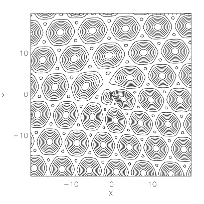
which implies that ${\bf\nabla.k_{1}=\nabla.k_{2}=0}$ hold. Since the wavevectors are gradients of the phases, it is clear that $\nabla\times{\bf k_{1}}=\nabla\times{\bf k_{2}}=0$ also hold, and that $\nabla^{2}\Theta_{1}=\nabla^{2}\Theta_{2}=0$. The solutions of these equations are the harmonic defects catalogued in [8]. Despite being energetically unreasonable, and hence looking somewhat unphysical, because they contain features at wavelengths which lie outside the stable region, they provide a good illustration of the topology of real defects. It is possible to construct a harmonic hepta-penta defect by positioning two harmonic dislocations [8] on top of each other, as shown in figure 1. The hepta-penta defect is the canonical defect of hexagons.

In the general nonvariational case, the Cross-Newell equations can be written

$$\tau(k_{1}^{2},k_{2}^{2},{\bf k_{1}.k_{2}})\Theta_{1T} = \alpha_{1}(k_{1}^{2},k_{2}^{2},{\bf k_{1}.k_{2}})\nabla.{\bf k_{1}}+\alpha_{2}(k_{1}^{2},k_{2}^{2},{\bf k_{1}.k_{2}}){\bf k_{1}}.\nabla k_{1}$$

$$+\alpha_{3}(k_{1}^{2},k_{2}^{2},{\bf k_{1}.k_{2}}){\bf k_{1}}.\nabla k_{2}+\alpha_{4}(k_{1}^{2},k_{2}^{2},{\bf k_{1}.k_{2}}){\bf k_{1}}.\nabla{\bf(k_{1}.k_{2})}$$

$$+\beta_{1}(k_{1}^{2},k_{2}^{2},{\bf k_{1}.k_{2}})\nabla.{\bf k_{2}}+\beta_{2}(k_{1}^{2},k_{2}^{2},{\bf k_{1}.k_{2}}){\bf k_{2}}.\nabla k_{1}$$

$$+\beta_{3}(k_{1}^{2},k_{2}^{2},{\bf k_{1}.k_{2}}){\bf k_{2}}.\nabla k_{2}+\beta_{4}(k_{1}^{2},k_{2}^{2},{\bf k_{1}.k_{2}}){\bf k_{2}}.\nabla{\bf(k_{1}.k_{2})},$$

$$\tau(k_{2}^{2},k_{1}^{2},{\bf k_{1}.k_{2}})\Theta_{2T} = \alpha_{1}(k_{2}^{2},k_{1}^{2},{\bf k_{1}.k_{2}})\nabla.{\bf k_{2}}+\alpha_{2}(k_{2}^{2},k_{1}^{2},{\bf k_{1}.k_{2}}){\bf k_{2}}.\nabla k_{2}$$

$$+\alpha_{3}(k_{2}^{2},k_{1}^{2},{\bf k_{1}.k_{2}}){\bf k_{2}}.\nabla k_{1}+\alpha_{4}(k_{2}^{2},k_{1}^{2},{\bf k_{1}.k_{2}}){\bf k_{2}}.\nabla{\bf(k_{1}.k_{2})}$$

$$+\beta_{1}(k_{2}^{2},k_{1}^{2},{\bf k_{1}.k_{2}})\nabla.{\bf k_{1}}+\beta_{2}(k_{2}^{2},k_{1}^{2},{\bf k_{1}.k_{2}}){\bf k_{1}}.\nabla k_{2}$$

$$+\beta_{3}(k_{2}^{2},k_{1}^{2},{\bf k_{1}.k_{2}}){\bf k_{1}}.\nabla k_{1}+\beta_{4}(k_{2}^{2},k_{1}^{2},{\bf k_{1}.k_{2}}){\bf k_{1}}.\nabla{\bf(k_{1}.k_{2})}.$$

In contrast to the variational case, these equations cannot in general be reduced to flux-divergence form, and hence it cannot be assumed that such general hexagonal patterns will have defects whose topology is given by that of harmonic defects.

7 Conclusion

This paper has derived the Cross-Newell equations for triangles and hexagons in a general real gradient system. The resulting equations can be put into flux-divergence form, indicating that the topology of defects of such a hexagonal pattern can be described by that of harmonic defects [8]. The general nonvariational case, however, is not flux-divergent. In both cases, the phase stability boundaries and modes of instability for general distorted hexagons and triangles can be recovered from the Cross-Newell equations.

An explicit analytical form for the Cross-Newell equations is found for both hexagons and triangles in the case where the governing equations are generalisations of the corresponding complex amplitude equations.

This work suggests avenues for further investigation. In particular, it would be interesting to analyse the Cross-Newell equations in a general nonvariational system, and also to integrate the phase equations numerically in order to make a comparison with an integration of the full governing equations, for example in order to compare the regions of stability of hexagons. A further interesting possibility is to use the Cross-Newell equations to investigate the simultaneous occurrence of up- and down-hexagons [15]. These avenues will form the basis of future work.

Acknowledgements

The author would like to thank Alan Newell and Thierry Passot for interesting and helpful discussions.

This work was supported by King’s College, Cambridge.

Figure 1: A harmonic hepta-penta defect. The figure shows contours of $f({\bf X})=\cos\Theta_{1}+\cos\Theta_{2}+\cos\Theta_{3}$, where $\Theta_{1}=R\cos(\alpha+\pi/2)-(\alpha+\pi/2)$, $\Theta_{2}=R\cos(\alpha+\pi/6)-(\alpha+\pi/6)$, $\Theta_{3}=-\Theta_{1}-\Theta_{2}$, and where ($R$, $\alpha$) are polar coordinates for ${\bf X}$.

References

- [1] H. Benard, Rev. Gen. Sci. Pures Ap. 11, 1261 (1900).
- [2] H. Benard, Rev. Gen. Sci. Pures Ap. 11, 1309 (1900).
- [3] H. Benard, Ann. Chim. Phys. 23, 62 (1901).
- [4] F. Melo, P.B. Umbanhowar and H.L. Swinney, Phys. Rev. Lett. 21, 3838 (1995).
- [5] P.B. Umbanhowar, F. Melo and H.L. Swinney, Physica A 249, 1 (1998).
- [6] L.R. Morris and W.C. Winegard, J. Crystal Growth 5, 361 (1969).
- [7] M.C. Cross and A.C. Newell, Physica D 10, 299 (1984).
- [8] T. Passot and A.C. Newell, Physica D 74, 301 (1994).
- [9] M. Assenheimer and V. Steinberg, Phys. Rev. Lett. 76, 756 (1996).
- [10] R.B. Hoyle, Appl. Math. Lett. 8, 81 (1995).
- [11] R.B. Hoyle, in Time-Dependent Nonlinear Convection, edited by P.A. Tyvand (Comput. Math. Publications, Southampton, 1998).
- [12] M. Bestehorn, Phys. Rev. E 48, 3622 (1993).
- [13] A.C. Newell and J.A. Whitehead, J. Fluid Mech. 38, 279 (1969).
- [14] M. Golubitsky, J.W. Swift and E. Knobloch, Physica D 10, 249 (1984).
- [15] M. Assenheimer and V. Steinberg, Phys. Rev. Lett. 76, 756 (1996); G. Dewel et al, Phys. Rev. Lett. 74, 4647 (1995); R.M. Clever and F.H. Busse, Phys. Rev. E 53, R2037 (1996).