Bilateral symmetry breaking in a nonlinear Fabry-Perot cavity exhibiting optical tristability

Abstract

We show the existence of a region in the parameter space that defines the field dynamics in a Fabry-Perot cylindrical cavity, where three output stable stationary states of the light are possible for a given localized incident field. Two of these states do not preserve the bilateral (i.e. left-right) symmetry of the entire system. These broken-symmetry states are the high-transmission nonlinear modes of the system. We also discuss how to excite these states.

Symmetries are at the backbone of physical theories. In Hamiltonian systems, symmetries are related to conserved quantities through Noether’s theorem, and they provide us with a powerful tool to understand Nature. The left-right symmetry of the fundamental laws of Nature (apart from the nonconservation of parity for the weak interaction) is a well-known fact [1]. In particular, the electromagnetic interaction possesses this symmetry at the fundamental level. However, there is no reason why an invariance of the evolution equations should be an invariance of the stationary states of the system [2]. In fact, most of the time the state of really big systems does not have the symmetry of the laws which govern it [3]. Here in a simple symmetrical dynamical system with a symmetric localized driving source, we have found an example of the dynamical breaking of a discrete fundamental symmetry of the system, namely, its left-right, or bilateral, symmetry.

Shortly after the proposal and demonstration of nondissipative optical bistability using Fabry-Perot cavities [4, 5], the effect on the bistable behaviour of the transverse field amplitude profile of the fundamental mode of the cavity was taken into account [6]. Nonlinearity and diffraction can excite several transverse modes of the cavity, and this will considerably modify the dynamics of the light [7]. For high finesse cavities, when only one longitudinal mode of the cavity is excited, the dynamics can be described with a single scalar wave equation [8, 9], which facilitates numerical analysis and physical interpretation. In this paper, we restrict ourselves to this regime. Generally speaking, a great variety of light dynamics can be observed [10, 16]. Concerning bistability, it has been shown that diffraction gives rise to transverse instability in one of the two branches of the plane wave bistable regime [8]. This raises the question if bistability can exist at all when important transverse effects are taken into account. Some families of stationary solutions have been found [12], but their role in the dynamics of the light has not been discussed. Here we consider new families of stationary solutions with broken symmetry which are relevant to the dynamics of the light that we numerically observed, and we discuss their stability and excitation.

We consider a cylindrical Fabry-Perot cavity [13] filled with a self-focusing Kerr nonlinear medium, $n=n_{0}+n_{2}|E|^{2}$, where $n$ is the refractive index of the medium, $n_{0}$ is the low-power refractive index, $n_{2}>0$ is the nonlinear coefficient, and $E$ is the electric field inside the cavity (see Fig. 1). The cavity is driven by a gaussian beam $E_{i}$ with beam widths in the transverse $x$ and $y$ directions given by $w_{x}$ and $w_{y}$ ($1/e^{2}$ half width intensity). The concave mirror in the $y$-direction has a radius of curvature $R$, and the width $w_{y}$ is chosen so that the incident beam matches the linear Hermite-Gaussian mode of the cavity in the $y$-direction. Both mirrors have very high reflectivity $\cal{R}$, and the incident beam is assumed to have a Rayleigh range in the $x$ direction $z_{x}=\pi w_{x}^{2}n_{0}/\lambda_{0}$ much larger than the cavity length $L$. $\lambda_{0}$ is the light wavelength in vacuum. Under these conditions, only a single longitudinal mode of the cavity is excited and the electric field $E$ has the structure $E(x,y,z,t)\propto\Psi(x,t)\exp(-y^{2}/w_{y}^{2})\sin(k_{c}z)\exp(-i\omega t)+c.c.\,$, where $\Psi$ is the normalized complex field envelope inside the cavity, $\omega$ is the frequency of the input beam $E_{i}$, $t$ is the time and $k_{c}$ is the resonance wavenumber of the linear cavity. Only one transverse mode in the $y$ dimension is selected out by the use of the cylindrical cavity. The field transmitted by the system is proportional to $\Psi$ [14], which obeys the driven Ginzburg-Landau equation [8, 9]

$$\frac{\partial\Psi}{\partial\tau}=\frac{i}{2}\frac{\partial^{2}\Psi}{\partial\xi^{2}}-i\theta\Psi+i|\Psi|^{2}\Psi+\Gamma(\Psi_{d}-\Psi)$$ (1)

where $\Psi_{d}$ is the driving field, which is proportional to the incident field, $\xi=x/w_{x}$ is the normalized $x$ coordinate and $\tau=t/t_{0}$ is the normalized time. The normalizing factor $t_{0}$ is given by $t_{0}=2n_{0}z_{x}/c$, where $c$ is the velocity of light in vacuum. The normalized cavity detuning $\theta$ is given by $\theta=2\Delta kz_{x}$, where $\Delta k=k_{c}-k$ and the wavenumber $k$ is $k=n_{0}\omega/c$. The amplitude decay rate $\Gamma$ is $\Gamma=({\cal T}+\alpha L)z_{x}/L$, where ${\cal T}=1-{\cal R}$ is the transmissivity of each mirror, and $\alpha$ is the loss coefficient of the material filling the cavity. The normalized amplitude $q$ of the driving field ($q\equiv\Psi_{d}(0)$), the normalized cavity detuning $\theta$, and the amplitude decay rate $\Gamma$ define the parameter space that determines the dynamics of the light in the Fabry-Perot etalon.

Let us consider a laser light that excites ${}^{85}{\rm Rb}$ atoms in their D₂ transition near $\lambda_{0}=780$ nm to provide a resonantly-enhanced optical nonlinearity. The mirror reflectivity is $\cal{R}$=0.995 and the cavity length $L=2$ mm. The intracavity loss is $\alpha\simeq 0.1$ dB/cm and the linear refractive index is taken to be $n_{0}\simeq 1$. A beam width $w_{x}\simeq 100\,\mu$m corresponds to $\Gamma\simeq 0.15$, and $\theta\simeq 0.4$ corresponds to a cavity frequency detuning $\Delta f\simeq 240$ MHz. The Rayleigh range in the $x$ direction is $z_{x}\simeq 40$ mm. The mode beam waist in the $y$ direction [15] is $w_{y}=\sqrt{g^{2}\lambda L/n_{0}\pi(1-g)^{2}}$, where $g=1-L/R$. For $g=0.6$, we obtain $w_{y}\simeq 28\,\mu$m, that can be achieved through an appropriate cylindrical mode-matching lens. The maximum nonlinear refractive index change $\Delta n$ is given by $\Delta n=\lambda|\Psi|^{2}/4\pi z_{x}A$, where $A=3/2\sqrt{8}$ is a mode overlap factor given by the field profile in the $y$ and $z$ directions. For the parameters considered here, $\Psi\simeq 1$ corresponds to $\Delta n\simeq 3\times 10^{-6}$, which has been observed in a cylindrical Fabry-Perot experiment in rubidium vapor [16].

The time evolution of the field $\Psi$, as described by Eq. (1), results from the interplay between different processes: transverse effects arising from the diffraction (second derivative) term in the wave equation, self-focusing due to the nonlinearity, energy input due to the driving field and energy loss due to the finite transmissivity of both mirrors. The actual values of the parameters $\{\Gamma,\theta,q\}$, will determine the influence on light dynamics of every one of the above mentioned processes. For large beam width, we have $\Gamma$,$\theta\gg 1$, so transverse effects are expected to be negligible in this limit. For small beam width, but large enough in order to be in the regime of validity of Eq. (1), the different competing processes depicted above are comparable. This is the regime we are considering in this paper. We will see that there is a region in parameter space where three possible output states with different broken and unbroken symmetries can be excited, and under appropriate circumstances, all stable output states can be excited. In all our considerations we will restrict ourselves to the case $\theta>0$, corresponding to a red-detuning of the laser from the cavity resonance. Finally, we point out that the total energy inside the cavity and the transmitted beam power are both proportional to $I=\int_{-\infty}^{\infty}|\Psi|^{2}\,d\xi$, and this varies at a rate

$$\frac{dI}{dt}=-2\Gamma\int_{-\infty}^{\infty}|\Psi|^{2}\,d\xi+\int_{-\infty}^{\infty}[\Psi^{*}\Psi_{d}+\Psi\Psi_{d}^{*}]\,d\xi$$ (2)

Thus Eq. (1) corresponds to a non-conservative system.

Let us first review the main results for the stability of plane wave solutions against transverse perturbations [8]. In the plane wave limit, when the second derivative of the field in Eq. (1) is neglected, the curve $|\Psi_{0}|-\Psi_{d}$, where $\Psi_{0}$ are the stationary plane wave solutions, is single-valued for $\theta<\sqrt{3}\Gamma$, whereas for $\theta>\sqrt{3}\Gamma$, is S-shaped and can lead to bistability. Stationary plane-wave solutions are unstable against transverse perturbation when both conditions $|\Psi_{0}|^{2}>\Gamma$ and $|\Psi_{0}|^{2}>\theta/2$ are fulfilled. Since the upper branch of the S-shaped curve $|\Psi_{0}|-\Psi_{d}$ always begins at $|\Psi_{0}|^{2}>2\,\theta/3$, it turns out that the upper branch is always unstable against transverse perturbation. This raises the question whether or not bistability exists at all when one takes into account the transverse structure of the beams.

For that purpose, we first look for stationary solutions of Eq. (1). We set $\partial\Psi/\partial\tau=0$, and solve the corresponding ordinary differential equation with a Newton-Raphson scheme [17]. Note that contrary to travelling wave configurations, where stationary solutions are related to a nonlinear wavenumber shift [18], in the cavity configuration this is not the case, since the presence of the driving field makes Eq. (1) no longer invariant under a global phase change. We do not explore all the variety of stationary solutions that Eq. (1) can support. Instead, we restrict ourselves to the stationary solutions that will play a role in our discussion of bistability. We plot in Fig. 2 families of stationary solutions corresponding to $\Gamma=0.15$ and $\theta=0.4$. Stationary solutions plotted in Fig. 2 can be divided into two families. The curve labeled $S$ corresponds to symmetric solutions $\Psi_{0}(\xi)$, such that $\Psi_{0}(\xi)=\Psi_{0}(-\xi)$. The curve labeled $B$ corresponds to to a pair of broken-symmetry solutions, $\Psi_{0}(\xi)$ and $\Psi_{0}(-\xi)$. The curve $S$ has three branches defined by the sign of the slope of the curve in the figure, and we will refer to them as lower, middle, and upper branches. Figure 3 shows the amplitude profiles of two stationary solutions, one with broken symmetry and the other with unbroken symmetry. Note the breaking of the left-right symmetry of the output field relative to that of the drive, for the broken-symmetry state.

To investigate the stability of the stationary solutions plotted in Fig. 2, we solve Eq. (1) with a split-step Fourier Transform algorithm [19]. We take as input some selected slightly perturbed stationary solution $\Psi(\xi,\tau=0)=\Psi_{0}(\xi)\left[1+v(\xi)\right]$, where $v(\xi)$ is a complex gaussian random variable for every value of the transverse coordinate with mean $\mu=0$ and typical deviation $\sigma=0.01$, for both the real and imaginary parts. The perturbative noise will seed any instability present in the system. Since some of the stationary solutions have broken symmetry, in order to monitor the time evolution of the field, in addition to the peak amplitude, we will also follow the centroid $\bar{\xi}$, defined as

$$\bar{\xi}(\tau)=\frac{\int_{-\infty}^{\infty}\xi|\Psi(\xi,\tau)|^{2}}{\int_{-\infty}^{\infty}|\Psi(\xi,\tau)|^{2}}.$$ (3)

For a symmetric beam, $\bar{\xi}(\tau)=0$. After extensive numerical solutions, we find stable stationary solutions in the lower branch of curve $S$, and in curve $B$ below $q\simeq 1.48$. This means that the outcome of the simulations are the corresponding stationary solutions $\Psi_{0}$ in each case. Stationary solutions corresponding to all other parts of curves $S$ and $B$ have been found to be unstable. In some cases, the stability analysis leads to one or the other of the two corresponding stable stationary solutions for a given amplitude of the driving field, which one depending on the noise. In other cases, the output is a time-varying pattern that depends on the particular value of the peak amplitude of the driving field. In most cases, when the stationary solution of the lower branch of curve $S$ is not excited, the output of simulations always show that the beam does not preserve the bilateral symmetry of the driving field. For values of the peak amplitude of the driving field $1.37<q<1.48$, there are three stable stationary solutions. The one corresponding to the lower branch of curve $S$, possesses an unbroken symmetry, and the transmissivity, defined as the ratio of the output beam power to the incident beam power, is low ($\simeq 1\%$). The pair of solutions corresponding to curve $B$, one displaced to the left, the other to the right of the drive beam by equal amounts, possesses broken symmetry. The transmissivity of this pair of solutions is remarkably high ($\simeq 75\%$). Thus the nonlinear Fabry-Perot cavity can be viewed as a nonlinear transmission device which selects out the broken-symmetry solutions as the high-transmission modes of the system.

Numerical simulations of Eq. (1) show that the symmetric state in the lower branch of curve $S$ can be excited after switching on the driving field with the appropriate amplitude of the driving field. In order to excite the broken-symmetry states, a route to bistability has to be properly devised. Which one of the two broken-symmetry states is actually excited in the numerical simulations shown in Figs. 4 and 5, depends on round-off noise, and the method of excitation. One method is to tune the amplitude of the driving field in a step-like way to a value $q>1.98$, so that a time-varying intermediate output state associated with curve $B$ is excited. Then the amplitude of the driving field $q$ is reset to the value where the broken-symmetry state is stable. We plot an example of such route to tristability in Fig. 4. Note the delay on the onset of the spontaneous symmetry breaking from the time the drive is switched down. The actual excitation of the broken-symmetry state depends on the characteristics of the intermediate unstable state that is excited, and on the duration of the round-trip time around the hysteresis loop. Another way to excite the stable state in curve $B$, it is to switch on the driving field and then to slowly ramp it down. Figure 5 show the actual excitation of both the symmetric and broken-symmetry states by this method.

We anticipate that these results, which we have obtained at the nonlinear classical field level, should be related to the scattering resonances of the underlying quantum field theory, in view of the correspondence principle.

This work has been supported by the Spanish Government under contract PB95-0768. Juan P. Torres is grateful to the Spanish Government for funding of his sabbatical leave through the Secretaría de Estado de Universidades, Investigación y Desarrollo. Jack Boyce and Raymond Chiao acknowledge support of the ONR and the NSF. We would also like to thank Eric Bolda, John Garrison, Morgan W. Mitchell, and Ewan Wright for very helpful discussions.

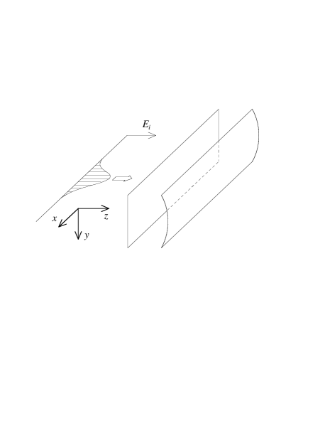
FIG. 1.: Geometry of the cylindrical Fabry-Perot cavity.

FIG. 2.: Families of stationary solutions. Curves labelled $S$ correspond to symmetric solutions, and curve labelled $B$ corresponds to broken-symmetry solutions. Parameters: $\Gamma=0.15$ and $\theta=0.4$.

FIG. 3.: Amplitude profiel of stationary solutions from the $S$ and $B$ curves. Parameters: $\Gamma=0.15$, $\theta=0.4$ and $q=1.45$. Solid line: amplitude profile of the field. Dotted line: amplitude profile of the driving field. Note the breaking of left-right symmetry for $B$.

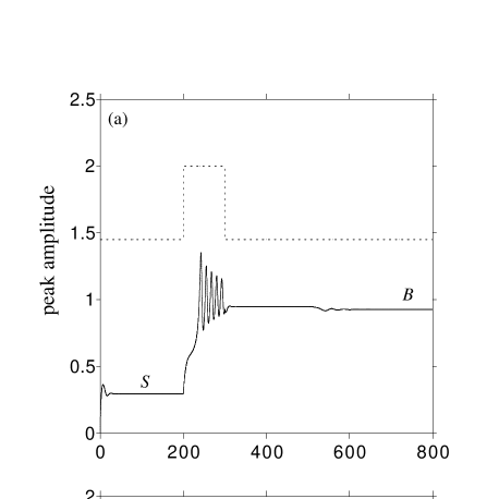
FIG. 4.: Step-like excitation of two stable states for $q=1.45$. (a) Peak amplitude and (b) centroid. Parameters: $\Gamma=0.15$, $\theta=0.4$ and $q=1.45$. $S$ corresponds to the excitation of the stationary solution in the lower branch of curve $S$, $B$ corresponds to the excitation of the stationary solution in curve $B$. Solid line: field. Dotted line: amplitude and centroid of the driving field. Note the delay in the onset of spontaneous symmetry breaking.

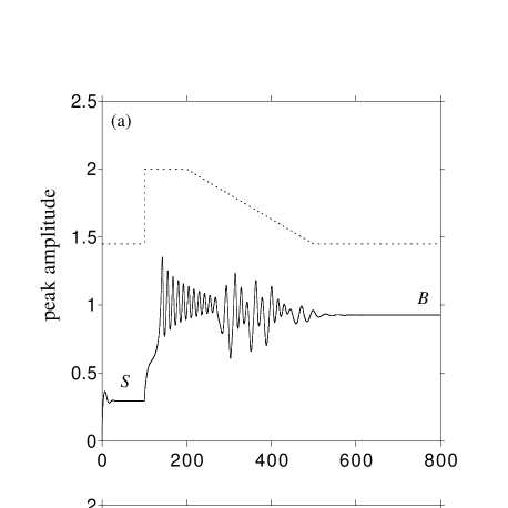
FIG. 5.: Ramp-like excitation of two stable states for $q=1.45$. (a) Peak amplitude and (b) centroid. Parameters: $\Gamma=0.15$, $\theta=0.4$ and $q=1.45$. $S$ corresponds to the excitation of the stationary solution in the lower branch of curve $S$, and $B$ corresponds to the excitation of the stationary solution in curve $B$. Solid line: field. Dotted line: amplitude and centroid of the driving field.

REFERENCES

- [1] T.D. Lee, Particle Physics and Introduction to Field Theory, (Harwood Academis Publishers, Amsterdam, 1988).
- [2] S. Coleman, Aspects of Symmetry, (Cambridge University Press, Cambridge, 1985).
- [3] P.W. Anderson, Science, 177 393 (1972).
- [4] H.M. Gibbs, S.L. McCall and T.N.C. Venkatesan, Phys. Rev. Lett., 36 1135 (1976).
- [5] F.S. Felber and J.H. Marburger, Appl. Phys. Lett., 28, 731 (1976).
- [6] J.H. Marburger and F.S. Felber, Phys. Rev. A, 17, 335 (1978).
- [7] W.J. Firth and E.M. Wright, Phys. Lett., 92, 211 (1982); Opt. Comm., 40, 233 (1982).
- [8] L.A. Lugiato and R. Lefever, Phys. Rev. Lett., 58, 2209 (1987).
- [9] M. Haelterman, M.D. Tolley and G. Vitrant, J. Appl.Phys., 67, 2725 (1990).
- [10] Y.I. Balkarei,M.G. Evitkhov, M.I. Elinson, A.S. Kogan and V.S. Posvyanskii, Quantum Electronics, 25, 641, (1995).
- [11] J. Boyce and R. Chiao, Phys. Rev. A, 59, 3953 (1999).
- [12] M. Haelterman, G. Vitrant and R. Reinisch, J. Opt. Soc. Am. B, 57, 1309 (1990); J. Opt. Soc. Am. B, 57, 1319, (1990).
- [13] I.H. Deutsch, R. Chiao and J.C. Garrison, Phys. Rev. Lett, 69, 3627 (1992).
- [14] H. Haus, Waves and Fields in Optoelectronics, (New York, Prentice-Hall, 1980).
- [15] P. Milonni and J.H. Eberly, Lasers, (John Wiley and sons, New York, 1988).
- [16] J. Boyce, J.P. Torres and R. Chiao, Opt. Lett., submitted.
- [17] W.H. Press, S.A. Teukolski, W.T. Vetterling and B.T. Flannery, Numerical Recipes in Fortan 77: the Art of Scientific Computing, (Cambridge, Cambridge University Pres, 1992).
- [18] N.N. Akhmediev and A. Ankiewicz, Solitons: Nonlinear Beams and Pulses, (Chapman-Hall, London, 1998).
- [19] G.P. Agrawal, Nonlinear Fiber Optics, (Academic Press, New York, 1989).