[

Crystallization Kinetics in the Swift–Hohenberg Model

Abstract

It is shown numerically and analytically that the front propagation process in the framework of the Swift-Hohenberg model is determined by periodic nucleation events triggered by the explosive growth of the localized zero-eigenvalue mode of the corresponding linear problem. We derive the evolution equation for this mode using asymptotic analysis, and evaluate the time interval between nucleation events, and hence the front speed. In the presence of noise, we derive the velocity exponent of “thermally activated” front propagation (creep) beyond the pinning threshold.

]

One of fundamental models of pattern formation far from equilibrium is the Swift-Hohenberg (SH) equation [1]. Despite relative simplicity of this model, and a serious limitation related to the fact that it is of the gradient type, it gives rise to a remarkably large variety of solutions. The SH equation has been intensively studied in the past as a paradigm model of pattern formation in large aspect ratio systems. [1, 2]. More recent computations brought attention to the propagation of fronts between uniform stationary states of this equation and coarsening [3]. The computations have also demonstrated formation of stationary solitons, i.e. stable localized objects in the form of a domain of one phase sandwiched inside another phase [3]. The interest was supported by applications of the SH model to marginally unstable optical parametric oscillators (OPO) [4], and more numerical computations, leading to similar conclusions, were carried out in this context [5]. The SH model has also served as a convenient testing tool for the problem of pattern propagation into an unstable trivial state [6, 7]. It is the purpose of this Letter to elucidate another aspect of pattern formation that can be modeled by the SH equation: coexistence between a pattern and a uniform state and stick-and-slip motion of interphase boundary which can be thought of as a particular kind of crystallization or melting.

We shall write the basic equation in the form

$$u_{t}=-(1+\nabla^{2})^{2}u+\epsilon u-u^{3}.$$ (1)

At $\epsilon>0$ the trivial state $u=0$ undergoes supercritical stationary bifurcation leading to a small-amplitude pattern with unit wavenumber $k$. The band of unstable wavenumbers widens with growing $\epsilon$, until it reaches the limiting value $k=0$, which signals the appearance of a pair of nontrivial uniform states, $u=\pm\sqrt{\epsilon-1}$. The two symmetric states are stable to infinitesimal perturbations at $\epsilon>\frac{3}{2}$. At still higher values of $\epsilon$, a variety of metastable states become possible: (1) a kink separating the two symmetric nontrivial uniform states (Fig. 1a); (2) a semi-infinite pattern, coexisting with either of the two nontrivial uniform states; (3) a finite patterned inclusion, sandwiched, either symmetrically or antisymmetrically, between semi-infinite domains occupied by nontrivial uniform states [8]; (4) a soliton (Fig. 1b) in the form of an island where one of the uniform states is approached, immersed in the infinite region occupied by the alternative state; the basic soliton “atom” can be viewed as a single period of the pattern immersed in a uniform state.

FIG. 1.: Stationary solutions to Eq. (1) for $\epsilon=1.78$. (a) kink solution connecting $u=\pm\sqrt{\epsilon-1}$; (b) 1D localized solution (solid line) and radially-symmetric solution to Eq. (1) (dashed line).

The energy of the uniform state is higher than that of the regular pattern with the optimal wavenumber at $\epsilon<6.287$ [10]. In spite of the difference between the energies of the uniform and patterned state, the interface between them remains immobile at moderate and large values $\epsilon$, and a multiplicity of localized states is linearly stable. The pattern propagation into a metastable uniform state or the reverse ”melting” process at $\epsilon\gg 1$ is impeded by the self-induced pinning attributed to the oscillatory character of the asymptotic perturbations of the uniform state, characterized by the complex wavenumber $k^{2}=-1\pm i\sqrt{2\epsilon-3}$. As $\epsilon$ decreases, the stationary localized solutions lose stability and give rise to propagating solutions.

We shall show in this Letter that the front propagation process can be described in terms of periodic nucleation events triggered by explosive growth of the localized zero-eigenvalue mode of the corresponding linear problem. Using asymptotic analysis, we shall derive the evolution equation for this mode which allows us to estimate the time interval between the nucleation events and hence the front speed. We shall also study the “thermally activated” front propagation (creep) at $\epsilon>\epsilon_{c}$ and derive the creep velocity exponent.

We performed numerical study of Eq.(1) in one spatial dimension at various values of $\epsilon$. We found that the depinning transition for the single soliton occurs at $\epsilon\approx 1.74$. The depinning threshold increases with the size of the patterned cluster, rapidly converging the limiting value $\epsilon=\epsilon_{c}\approx 1.7574...$ for the semi-infinite pattern. Figure 2 shows propagation of the semi-infinite pattern into a uniform stable state at $\epsilon=1.75$. The front propagation takes the form of well separated in time periodic nucleation events of new “atoms” of the “crystalline” state at the front. Between successive nucleation events, the solution remains close to the stationary semi-infinite pattern found at $\epsilon_{c}$. This process resembles crystallization in equilibrium solids, with the important distinction that the new “atoms” are created directly from the metastable “vacuum” state. The time between consecutive nucleation events diverges as $\epsilon$ approaches the pinning threshold [9]. Figure 3 presents the average front speed as a function of $\epsilon-\epsilon_{c}$. This function can be fitted by $V=V_{0}\sqrt{\epsilon_{c}-\epsilon}$, with $V_{0}=2.292$.

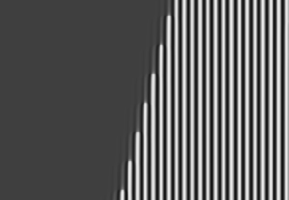
FIG. 2.: The space-time plot of the switching wave propagation into the stable uniform phase at $\epsilon=1.757$. The horizontal axis is spatial coordinate, and the vertical axis is time. The system size is 200 (4096 mesh points), the time span is 200.

FIG. 3.: The average front speed as a function of the control parameter $\epsilon$ near the critical point $\epsilon_{c}=1.7574..$. Points represent numerics, the dashed line is the best fit $V=2.29(\epsilon_{c}-\epsilon)^{1/2}$ and the dot-dashed line is the theoretical prediction $V=1.80(\epsilon_{c}-\epsilon)^{1/2}$.

At $\delta=\epsilon-\epsilon_{c}>0$, the immobile front solution $u_{0}(x,\epsilon)$ is linearly stable. Numerical stability analysis shows that there exists an exponentially decaying mode $u_{1}(x,\epsilon)$ localized at the front with negative eigenvalue $\lambda_{s}$ which approaches zero as $\delta^{1/2}$. In addition, there is also an unstable front solution and a corresponding mode with positive eigenvalue $\lambda_{u}$ which also approaches zero as $\delta^{1/2}$. At the pinning threshold, these two solutions collide and disappear via a saddle-node bifurcation. The stationary front solution $U_{0}(x)\equiv u_{0}(x,\epsilon_{c})$ and the corresponding mode structure $U_{1}(x)\equiv u_{1}(x,\epsilon_{c})$ are shown in Fig.4. In the inset, we show the stable and unstable eigenvalues $\lambda_{s,u}$ as functions of $\epsilon$. At $\epsilon<\epsilon_{c}$, the front solution becomes non-stationary. Nonetheless, at $|\delta|\ll 1$, the numerical study suggests that the solution remains close to the stationary front solution $U_{0}(x)$ all the time except short intervals when a new roll nucleates.

FIG. 4.: The stationary structure $U_{0}(x)$ (solid line) and the corresponding localized zero mode $U_{1}(x)$ (dashed line) at $\epsilon=\epsilon_{c}$. Inset: eigenvalues of the stable and unstable localized modes of the stationary front solutions at $\epsilon>\epsilon_{c}$.

The process of front propagation can be analyzed within the framework of perturbation theory near the critical value $\epsilon=\epsilon_{c}$. At $|\delta|\ll 1$, we can present the front solution in the form

$$u(x,t)=U_{0}(x)+|\delta|^{1/2}u_{1}(x,t),$$

where $U_{0}(x)$ is the stationary front solution at $\delta=0$ and $|\delta|^{1/2}u_{1}(x,t)$ is a small correction. This solution is uniformly valid at small positive $\delta$; it is also valid during quasi-stationary phases (away from nucleation events) for small negative $\delta$. Plugging this ansatz in Eq.(1), we obtain

$$\partial_{t}u_{1}=L[U_{0}]u_{1}-|\delta|^{1/2}\left[3U_{0}u_{1}^{2}-\mbox{sign}(\delta)U_{0}\right]+...,$$ (2)

where $L[U_{0}]\equiv\epsilon_{c}-3U_{0}^{2}-(1+\nabla^{2})^{2}$ is the linearized SH operator at $\epsilon_{c}$. In the lowest order in $\delta$, Eq.(2) yields the linear equation $\partial_{t}u_{1}=L[U_{0}]u_{1}$. This equation is always satisfied by the stationary translational mode $U_{0}^{\prime}(x)$. In addition, the linearized operator $L[U_{0}]$ has a localized neutral eigenmode $U_{1}$ (found numerically above, see Figure 4). Since all other eigenmodes have negative eigenvalues, the evolution of the system close to the bifurcation point can be reduced to single-mode dynamics [11]. Therefore in the lowest order we can write $u_{1}(x,t)=a(t)U_{1}(x)$, where $a(t)$ is the amplitude of the zero mode.

Close to the bifurcation threshold $\partial_{t}u_{1}=\dot{a}U_{1}$ can be treated as perturbation. Therefore, in the second order we derive

$$L[U_{0}]u_{2}=\dot{a}U_{1}+|\delta|^{1/2}\left[3a^{2}U_{0}U_{1}^{2}-\mbox{sign}(\delta)U_{0}\right].$$ (3)

Eq. (3) has a bounded solution if its r.h.s. is orthogonal to the zero mode $U_{1}$ of the operator $L$. This results in the solvability condition for the amplitude $a$:

$$\alpha\,\dot{a}=|\delta|^{1/2}\left[\mbox{sign}(\delta)\beta-\gamma a^{2}\right],$$ (4)

where

$$\alpha=\int_{-\infty}^{\infty}U_{1}^{2}dx,\;\;\beta=\int_{-\infty}^{\infty}U_{1}U_{0}dx,\;\;\gamma=3\int_{-\infty}^{\infty}U_{1}^{3}U_{0}dx.$$

At $\delta>0$, $a(t)$ reaches a stationary amplitude $a_{0}=(\beta/\gamma)^{1/2}$. This value corresponds to the difference between the stable front solutions at $\epsilon$ and $\epsilon_{c}$. At small negative $\delta$, Eq.(4) describes explosive growth of $a$, which passes from $-\infty$ to $\infty$ in a finite time $\tau_{e}=\pi\alpha/(|\delta|\beta\gamma)^{1/2}$. This explosion time gives an upper bound for the period between the nucleation events, after which the whole process repeats. The front speed is found as $V=\Lambda/\tau_{e}$, where $\Lambda$ is the asymptotic spatial period of the pattern selected by the process of roll nucleation, and $\tau_{e}$ is the time interval between nucleation events. Our calculations give the value: $V=1.8|\delta|^{1/2}$. This scaling is in a good qualitative agreement with the results of the numerical simulations, see Fig.3. However, the prefactor $1.8$ is noticeably lower (about 25%) than the corresponding value $V_{0}=2.29$ obtained by numerical simulation of Eq. (1).

Let us discuss a possible reason for the discrepancy. Our numerical simulations show that the nucleation events produce slowly-decaying distortions behind the moving front. These distortions may effectively “provoke” a consequent nucleation event by creating an initial perturbation of the zero mode $U_{1}(x)$. It will lead to an increase of the front velocity. Although we have evidence for the importance of this effect, a systematic treatment of this process is very complicated and goes beyond perturbation theory.

Effect of noise.

Let us consider the effect of weak additive noise $\eta(x,t)$ in the r.h.s. of Eq. (1). For simplicity we assume that $\eta$ is delta-correlated noise with the intensity (temperature) $T$:

$$\langle\eta(x,t)\eta(x^{\prime},t^{\prime})\rangle=T\delta(x-x^{\prime})\delta(t-t^{\prime}).$$

In the presence of noise, there is no sharp threshold for the onset of motion at $\epsilon<\epsilon_{c}$. Instead, thermally-activated motion (creep) occurs at $\epsilon>\epsilon_{c}$ (see Fig. 5). In this case the average creep velocity is determined by the intensity of noise. For $\epsilon<\epsilon_{c}$ the noise will slightly increase the speed of the front. In contrast to the deterministic motion, the intervals between consecutive nucleation events are random.

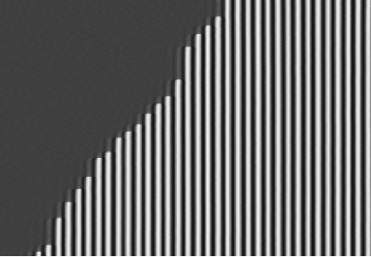
FIG. 5.: The space-time plot of the switching wave propagation triggered by white noise with the temperature $T=0.00042$ at $\epsilon=1.758>\epsilon_{c}$. The horizontal axis is spatial coordinate, and the vertical axis is time. The system size is 200 (4096 mesh points), the time span is 1000.

In order to estimate the effect of the noise at $\delta>0$, we will treat $\eta$ as small perturbation. In this analysis, we shall not introduce scaling explicitly, since the scaling of noise that is comparable by its effect with deterministic perturbations cannot be determined a priori. Following the lines of the above analysis, we project noise at the zero mode to obtain the solvability condition

$$\alpha\,\dot{a}=\delta^{1/2}(\beta-\gamma a^{2})+\delta^{-1/2}\tilde{\eta}(t),$$ (5)

where $\tilde{\eta}(t)=\int_{-\infty}^{\infty}\eta(x,t)U_{1}(x)dx$. For $T=0$, Eq. (5) has a stable fixed point $a_{s}=\sqrt{\beta/\gamma}$ and an unstable one $a_{u}=-\sqrt{\beta/\gamma}$. At $a<a_{u}$, one has explosive growth of the solution to Eq. (5), while $a\to a_{s}$ at $a>a_{u}$. Thus, we have to estimate the probability $P$ for the amplitude of the zero mode $a$ to be smaller than $a_{u}$. This quantity can be derived from the corresponding Fokker-Planck equation for the probability density $p(a,t)$ [12]:

$$p_{t}=-\frac{\delta^{1/2}}{\alpha}\frac{\partial}{\partial a}\left[(\beta-\gamma a^{2})p\right]+\frac{T}{2\alpha\delta}\partial_{a}^{2}p,$$ (6)

where we used $\langle\tilde{\eta}^{2}\rangle=\alpha T$. This is the standard Kramers problem. The stationary probability $p(a)$ is given by

$$p\sim\exp\left[\frac{2\delta^{3/2}(\beta a-\gamma a^{3}/3)}{T}\right].$$ (7)

The probability $P$ is given by the integral $P=\int_{-\infty}^{a_{u}}p(x)dx$. For $T\ll\delta^{3/2}$, we can use the saddle-point method, which gives the following result:

$$P(a<a_{u})\sim\exp\left[-\frac{4\delta^{3/2}\beta^{3/2}}{3\gamma^{1/2}T}\right]=\exp\left[-\frac{0.57\delta^{3/2}}{T}\right].$$ (8)

Since the time between the nucleation events $\tau_{n}\sim 1/P$, we find that the velocity of the front in the stable region is given by $v\sim 1/\tau_{n}\sim\exp\left[-0.57\delta^{3/2}/T\right]$.

At very large $\epsilon>\epsilon_{0}=6.287$, the flat state $u=\pm\sqrt{\epsilon-1}$ has lower energy than the periodic state. Nevertheless, the uniform state does invade periodic state at any $\epsilon$ because of the strong self-induced pinning. With large-amplitude noise there will be some probability for the flat state to propagate towards periodic state by thermally-activated annihilation events at the edge of the periodic pattern, however t large $\epsilon$ the probability of annihilation at the edge is of the same order as that in the bulk of the patterned state. Thus, for very large $\epsilon$ and large $T$ we may expect melting of the periodic structure both on the edge and in the bulk.

The above results can be trivially extended to regular two-dimensional periodic structures (rolls) selected by the SH equation [1]. More interesting is the behavior of a 2$D$ hexagonal lattice which was predicted by weakly nonlinear analysis near the bifurcation of nontrivial uniform solutions at $\epsilon=\frac{3}{2}$ and found numerically [13]. We anticipate that propagation of the hexagonal structure into the uniform state will exhibit the same features of stick-and-slip motion as described above, and can be studied by similar methods. For SH equation (1) at $\epsilon>\frac{3}{2}$, hexagonal lattices coexist with roll patterns which have lower energy, so the front propagation may in fact give rise to rolls. However, the hexagons may become dominant in the modified SH equation with an added quadratic nonlinearity near $\epsilon=0$, where the robust “crystallization” of the hexagonal lattice is expected. The work on this subject is now in progress.

The authors thank the Max-Planck-Institut für Physik komplexer Systeme, Dresden, Germany for hospitality during the Workshop on Topological Defects in Non-Equilibrium Systems and Condensed Matter. ISA and LST acknowledge support from the U.S. DOE under grants No. W-31-109-ENG-38, DE-FG03-95ER14516, DE-FG03-96ER14592 and NSF, STCS #DMR91-20000. LMP acknowledges the support by the Fund for Promotion of Research at the Technion and by the Minerva Center for Nonlinear Physics of Complex Systems.

REFERENCES

- [1] M.C. Cross and P.C. Hohenberg, Rev. Mod. Phys. 65, 851 (1993).
- [2] H.S. Greenside and M.C. Cross, Phys. Rev. A 31, 2492 (1985)
- [3] K. Ouchi and H. Fujisaka, Phys. Rev. E 54, 3895 (1996).
- [4] P. Mandel, M. Georgiu, and T. Erneux, Phys. Rev. A 47, 4277 (1993).
- [5] K. Staliunas and V.J. Sánchez-Morcillo, Phys. Lett. A 241, 28 (1998).
- [6] G.T. Dee and W. van Saarloos, Phys. Rev. Lett. 60, 2641 (1988).
- [7] W. van Saarloos, Phys. Rev. A 39, 6367 (1989).
- [8] Finite patterned inclusions have been obtained in a modified SH equation including a quintic term by H. Sakaguchi and H.R. Brand, Physica D 97, 274 (1996).
- [9] The front dynamics is similar to that considered by I. Mitkov, K. Kladko, and J.E. Pearson, Phys. Rev. Lett.81, 5453 (1998). In our case, the pinning is, however , self-induced, whereas in the cited work it is caused by discrete sources.
- [10] A close value of was obtained in Ref. [3] using relaxation method. We obtained a more accurate estimate of and the corresponding optimal wavenumber by matching-shooting method for stationary Eq. (1). The above values were derived by comparing the energy of the uniform state with the energy of the periodic state with the optimal wavenumber.
- [11] The translational mode of course also has a zero eigenvalue. However, its mobility vanishes, since the friction factor is infinite, and therefore this mode can be excluded.
- [12] N.G. Van Kampen, Stochastic processes in physics and chemistry, Elsevier, 1997.
- [13] G. Dewel, S. Métens, M’F. Hilali, P. Borckmans and C.B. Price, Phys. Rev. Lett.74, 4647 (1995).