Soliton Interactions in Perturbed Nonlinear Schrödinger Equations

Abstract

We use multiscale perturbation theory in conjunction with the inverse scattering transform to study the interaction of a number of solitons of the cubic nonlinear Schrödinger equation under the influence of a small correction to the nonlinear potential. We assume that the solitons are all moving with the same velocity at the initial instant; this maximizes the effect each soliton has on the others as a consequence of the perturbation. Over the long time scales that we consider, the soliton amplitudes remain fixed, while their center of mass coordinates obey Newton’s equations with a force law for which we present an integral formula. For the interaction of two solitons with a quintic perturbation term we present more details since symmetries — one related to the form of the perturbation and one related to the small number of particles involved — allow the problem to be reduced to a one-dimensional one with a single parameter, an effective mass. The main results include calculations of the binding energy and oscillation frequency of nearby solitons in the stable case when the perturbation is an attractive correction to the potential and of the asymptotic “ejection” velocity in the unstable case. Numerical experiments illustrate the accuracy of the perturbative calculations and indicate their range of validity.

1 Introduction

This paper is concerned with the asymptotic behavior of solutions of the initial-value problem for the perturbed nonlinear Schrödinger equation (NLSE)

$$i\partial_{t}\psi+\frac{1}{2}\partial_{x}^{2}\psi+|\psi|^{2}\psi+p[\psi,\psi^{*}]=0\,,$$ (1)

subject to the initial condition $\psi(x,0)=\psi_{0}(x)$ for certain initial fields $\psi_{0}(x)$, in the limit when the perturbation term $p[\psi,\psi^{*}]$ becomes formally small. The unperturbed problem, when $p[\psi,\psi^{*}]\equiv 0$ in (1), is well-known to be solvable [1] by an inverse scattering transform, one consequence of which is the existence of finite energy soliton solutions that are dynamically stable and robust with respect to collisions. The unperturbed NLSE arises in two different physical situations in modern optics [2]. Firstly, for high-speed telecommunications, (1) describes the propagation of light wave-packets along an optical fiber. In this interpretation, $t$ is the spatial coordinate along the fiber and $x$ is the retarded time variable for the signal; accordingly the solitons of the unperturbed problem (and usually also the solitary waves of the perturbed problem, when they exist) are called temporal solitons. The suggestion by Hasegawa and Tappert in 1973 [3, 4] that temporal solitons, being immune to dispersion, might serve as bits in a high-speed data stream has since generated a large body of work, much of which is comprehensively reviewed in [5, 6]. Secondly, for photonic switching devices, (1) describes the stationary envelope of monochromatic light waves in a planar waveguide under the paraxial approximation. Here $x$ and $t$ are both spatial variables, with $t$ being the propagation direction and $x$ being the transverse direction; accordingly the solitons of the unperturbed problem are called spatial solitons.

In both of these applications, the cubic term $|\psi|^{2}\psi$ in (1) models the Kerr effect in which the refractive index of the material depends linearly on the local intensity of light. For weakly nonlinear effects, when intensities are not too large, this effect is dominant in isotropic materials like glass. This fact, along with the integrability afforded by neglecting $p[\psi,\psi^{*}]$, makes the unperturbed NLSE one of the most important models in modern optics.

Of course, real materials can have a complicated dependence of refractive index on intensity, for which the Kerr effect is only an idealization. Modeling such phenomena requires introducing corrections to the coefficient $|\psi|^{2}$ in the cubic term of the NLSE. The perturbative term $p[\psi,\psi^{*}]$ might also include corrections related to higher-order dispersion, the Raman effect, self-steepening of pulses, etc. In this paper we will consider only the influence of higher-order nonlinearity on solitons of the unperturbed NLSE. For spatial solitons in photorefractive media, such a perturbation can be the main factor influencing propagation. In particular, we take the perturbation in (1) in the form of a quintic term

$$p[\psi,\psi^{*}]=\sigma\epsilon^{2}|\psi|^{4}\psi\,,$$ (2)

where $\epsilon>0$ is a small parameter and $\sigma=\pm 1$.

In view of the possibility of using solitons as bits in optical fibers or dynamically controllable switches in planar waveguides, it is of some interest to determine the effect of such a perturbation on the solitons of the unperturbed problem. If one considers an initial condition $\psi_{0}(x)$ that is a “snapshot” of a simple soliton solution of the unperturbed problem, then there are many approaches available to study the perturbed evolution. Because the unperturbed soliton is stationary in some Galilean frame, the main effect of $p[\psi,\psi^{*}]$ will be an adiabatic adjustment of the soliton’s amplitude and phase parameters. This fact, together with the simplicity of the form of the soliton solution, means that direct perturbative methods can be used to study their slow evolution. In particular, variational methods and multiscale methods applied directly to (1) often give valid results. These perturbative methods are dynamical in origin and capture effects on finite but long scales. Other methods can be used to answer infinite time questions concerning the persistence of solitary waves. In fact in the presence of quite general perturbations solitary waves continue to exist for arbitrary $\epsilon$ [7, 8] and these can be expressed in closed form in some cases [2].

The presence of more than one soliton complicates the analysis. If the solitons are isolated then the field may be approximated as a sum of solitons plus a small error term, and the adiabatic coupling among the solitons may be calculated by several methods. Note that if the solitons are moving with respect to each other then they will always be in isolation except possibly for a short time. An early analysis of this kind was carried out by Gordon [9], who studied the exact two-soliton solution of the unperturbed NLSE for equal velocities. When the solitons are well-separated, there is an effective force between them (even in the unperturbed NLSE) that varies sinusoidally with their phase difference. This phase difference grows linearly in $t$ if the solitons differ in amplitude. The force is therefore zero on average [10] and one expects periodic motion. This is a physical explanation of the mathematical fact that the intensity $|\psi|^{2}$ of the exact two-soliton solution for equal velocities is a periodic function of $t$. An extension of this argument to perturbed problems was given by Ankiewicz [11], who obtained a simple description of soliton interactions with the use of complex averaged potentials. Again, the essential assumption is that the solitons are well-separated in $x$, so that the field may be approximated as a sum of solitons. If the solitons are close to each other, nonlinear interference effects cause the field to adopt a form very different from the linear superposition of individual solitons, and therefore a different approach is needed. Often, one turns to numerics to study the interactions of solitons in various media (see, for example, [12, 13, 14]) without the restriction of the solitons being isolated.

In the scattering transform domain, where the dynamics of the unperturbed NLSE are trivial, a state in which two solitons are close to each other in $x$ has the same spectrum as a state in which they are far apart. This suggests that for studying the influence of perturbations on multisoliton bound states (that is, several solitons traveling with the same velocity, represented by a collection of eigenvalues of the Zakharov-Shabat equations with the same real part) it is best to carry out the analysis in the transform domain using soliton perturbation theory [7, 15, 8]. With $p[\psi,\psi^{*}]\neq 0$, the evolution of the scattering data is no longer trivial, and thus the scope of possible dynamics in near-integrable systems like (1) is much greater than in the unperturbed NLSE, including effects like repulsion, attraction, and energy exchange among bound or colliding solitons. Other techniques that have been used to study these effects include the judicious use of conserved quantities [2], variational methods [16, 17], “equivalent particle” approaches [18, 19], and of course, numerics.

In this paper, we use soliton perturbation theory to study perturbations of the nonlinear potential in (1), for initial conditions $\psi_{0}(x)$ that are snapshots of multisoliton bound states of the unperturbed NLSE. With respect to treating the solitons in isolation, this is a worst-case scenario since in the unperturbed NLSE a tightly-bound state of solitons will remain so for all time. Nonetheless, it is a scenario of some interest, in particular for the quintic perturbation (2). If $\sigma=+1$, then it is known that the solution remains bound, and this case has been studied using conservation laws [20]. If $\sigma=-1$, then the bound state becomes destabilized. Recently it was shown [21] by simulations of (1) that the instability causes the bound state to divide into isolated solitons that are ejected from the origin with nonzero relative velocities. On the time scales over which this splitting occurs, the solitons do not appear to exchange energy. In mathematical terms, each eigenvalue in the bound state ensemble, originally confined to the imaginary axis (zero velocity), appears to slowly “grow” a real part while its imaginary part remains fixed. Once the solitons escape, they no longer interact and the velocities no longer change. The wave guidance properties of Y-junctions engineered from such splittings of spatial solitons have also been analyzed [22].

By considering the relative velocities to be small, we will find an integral formula that expresses the asymptotic velocity difference between a pair of initially co-propagating solitons destabilized by the quintic perturbation (2) with $\sigma=-1$. Along the way, we will write down a coupled system of differential equations that describes the interaction of any number of solitons under more general perturbations over long time scales. These equations are just Newton’s equations for a system of interacting particles in one space dimension; the particle coordinates have the interpretation of the soliton centers of mass. The force is translationally invariant, conserves the total momentum, and is also proportional to $\sigma$, so the forces giving rise to attraction and repulsion are related just by a change of sign. For the interaction of two solitons, the problem may be reduced to a single degree of freedom, the relative separation of the solitons. The force law scales simply with the (fixed) amplitudes, which have the interpretation of masses. The result is a one-parameter family of problems indexed by a normalized effective mass. If the separation is small in the attractive case $\sigma=+1$, the force is nearly linear and the frequency of motion becomes a function of the normalized effective mass. We calculate this frequency, a quantity that is connected with the vibrations of solitons that are infinitely close, a limit opposite to the well-separated case.

Our paper begins in §2 with a review of the theory of the scattering transform for the Zakharov-Shabat eigenvalue problem and of the inverse theory that holds in the reflectionless case. We also recall the derivation of the exact equations of motion in the transform domain corresponding to the perturbed NLSE (1). Then, in §3 we consider perturbations of the form $p[\psi,\psi^{*}]=\epsilon^{2}W(|\psi|^{2})\psi$ and apply multiscale perturbation theory to find asymptotic solutions of the equations of motion in the transform domain. The approximations are uniformly valid as $\epsilon\downarrow 0$ on expanding time intervals of length $\epsilon^{-1}$, and are given in terms of solutions of Newton’s equations for particles interacting in one dimension under a force law that has several universal features. In §4 we focus on the quintic perturbation (2) and study the interaction of two solitons. We reduce the problem to the motion of a single particle and then explicitly perform the averaging required to remove secular terms from the asymptotic expansion. This leaves the force law in the form of a 1D integral that we study numerically. We use it to compute the “ejection” velocity observed by Artigas et. al. [21] in the unstable case and the harmonic frequency of tightly-bound solitons in the stable case. Finally, we compare the results of perturbation theory with direct simulations of (1). The Appendix contains the more cumbersome formulae that nonetheless are among our main analytical results.

Regarding notation, we will use stars for complex conjugation, and matrices will be written with bold letters, except for the Pauli matrices

$$\sigma_{1}:=\left[\begin{array}[]{cc}0&1\\ 1&0\end{array}\right]\,,\hskip 21.68121pt\sigma_{2}:=\left[\begin{array}[]{cc}0&-i\\ i&0\end{array}\right]\,,\hskip 21.68121pt\sigma_{3}:=\left[\begin{array}[]{cc}1&0\\ 0&-1\end{array}\right]\,.$$ (3)

2 Exact Inverse Scattering Theory For The Perturbed NLSE

Here, we review the known inverse scattering theory for the Zakharov-Shabat eigenvalue problem to fix our notation. In general, we wish to consider (1) where $p[\psi,\psi^{*}]$ is a polynomial in $\psi$, $\psi^{*}$, and their $x$-derivatives. The field $\psi$ is taken to be in the Schwartz space as a function of $x$.

2.1 Scattering data.

We will work with the scattering transform of $\psi$, a map that associates to the complex field $\psi$ at each fixed time a set of “scattering data” from which $\psi$ can be reconstructed by inverting the map. As is well-known, the advantage of this is that the time evolution of the scattering data corresponding to the time evolution of $\psi$ is trivial when $p\equiv 0$. Consequently, when $|p|\ll 1$, this proves to be a useful setting for perturbation theory.

Fix $t$, and assume the complex function $\psi(x,t)$ to be given. For $\lambda\in{\mathbb{R}}$ denote by ${\bf M}^{\pm}(x,t,\lambda)$ the $2\times 2$ matrix solutions of the linear differential equation

$$\partial_{x}{\bf M}^{\pm}={\bf L}{\bf M}^{\pm}:=\left[\begin{array}[]{cc}-i\lambda&\psi\\ -\psi^{*}&i\lambda\end{array}\right]{\bf M}^{\pm}\,,$$ (4)

satisfying the boundary conditions ${\bf M}^{\pm}(x,t,\lambda)\exp(i\lambda\sigma_{3}x)\rightarrow{\mathbb{I}}$ as $x\rightarrow\pm\infty$ Since ${\bf L}$ is traceless, these boundary conditions guarantee that these matrices are unimodular for all $x$. For each $\lambda$ there can only be two linearly independent column vector solutions of (4); therefore there is a matrix ${\bf S}(t,\lambda)$, $\lambda\in{\mathbb{R}}$, the scattering matrix, such that

$${\bf M}^{-}(x,t,\lambda)={\bf M}^{+}(x,t,\lambda){\bf S}(t,\lambda)\,.$$ (5)

The first column of ${\bf M}^{-}(x,t,\lambda)$ and the second column of ${\bf M}^{+}(x,t,\lambda)$ turn out to be boundary values of analytic functions for $\Im(\lambda)>0$, while the second column of ${\bf M}^{-}(x,t,\lambda)$ and the first column of ${\bf M}^{-}(x,t,\lambda)$ are the boundary values of analytic functions for $\Im(\lambda)<0$. Adjoining the second column of ${\bf M}^{+}(x,t,\lambda)$ on the right of the first column of (5) and taking determinants gives

$$S_{11}(t,\lambda)=\det(M_{1}^{-}(x,t,\lambda),M_{2}^{+}(x,t,\lambda))\,,$$ (6)

which is therefore the boundary value of a function analytic for $\Im(\lambda)>0$. Likewise $S_{22}(t,\lambda)=\det(M_{1}^{+}(x,t,\lambda),M_{2}^{-}(x,t,\lambda))$ is the boundary value of a function analytic for $\Im(\lambda)<0$.

Fix $\lambda\in{\mathbb{R}}$. Then, from (4), ${\bf M}^{\pm*}=\sigma_{2}{\bf M}^{\pm}\sigma_{2}$, and thus ${\bf S}^{*}=\sigma_{2}{\bf S}\sigma_{2}$, so that $S_{22}=S_{11}^{*}$ and $S_{21}=-S_{12}^{*}$. In particular, this means that as an analytic function for $\Im(\lambda)<0$, $S_{22}(t,\lambda)=S_{11}(t,\lambda^{*})^{*}$. Also, for $\lambda\in{\mathbb{R}}$ the fact that $\det({\bf S})=1$ implies the normalization condition $|S_{11}|^{2}+|S_{12}|^{2}=1$.

The analytic function $S_{11}(t,\lambda)$ with $\Im(\lambda)>0$ may have zeros $\lambda_{1}(t),\dots,\lambda_{N}(t)$. The determinant formula (6) then shows that there exist complex numbers $\gamma_{1}(t),\dots,\gamma_{N}(t)$ such that

$$M_{2}^{+}(x,t,\lambda_{k}(t))=\gamma_{k}(t)M_{1}^{-}(x,t,\lambda_{k}(t))\,,\hskip 21.68121ptk=1,\dots,N\,.$$ (7)

The conjugation symmetry of ${\bf M}^{\pm}(x,t,\lambda)$ for $\lambda\in{\mathbb{R}}$, when extended to the complex plane, implies that at the complex conjugate points $\lambda_{k}(t)^{*}$ where $S_{22}(t,\lambda)$ vanishes, $M_{1}^{+}(x,t,\lambda_{k}(t)^{*})=-\gamma_{k}(t)^{*}M_{2}^{-}(x,t,\lambda_{k}(t)^{*})$, for $k=1,\dots,N$. Since $S_{11}(t,\lambda)\rightarrow 1$ as $\lambda\rightarrow\infty$ with $\Im(\lambda)>0$, Hilbert transform theory can be used in conjunction with the normalization condition to express $S_{11}(t,\lambda)$ for $\Im(\lambda)>0$ in terms of its zeros and the values of $S_{12}(t,\lambda)$ on the real axis [23]:

$$S_{11}(t,\lambda)=\left(\prod_{k=1}^{N}\frac{\lambda-\lambda_{k}(t)}{\lambda-\lambda_{k}(t)^{*}}\right)\exp\left(\frac{1}{2\pi i}\int_{-\infty}^{\infty}\frac{\log(1-|S_{12}(t,\mu)|^{2})}{\mu-\lambda}\,d\mu\right)\,.$$ (8)

The so-called “trace formulae” that equate certain functionals of the potential $\psi$ to functionals of the scattering data will be useful below. In particular, we will use the formula:

$$P[\psi,\psi^{*}]:=\int_{-\infty}^{\infty}\Im(\psi\partial_{x}\psi^{*})\,dx=\frac{1}{2\pi}\int_{-\infty}^{\infty}\mu\log(1-|S_{12}(t,\mu)|^{2})\,d\mu-\sum_{k=1}^{N}\Im(\lambda_{k}(t)^{2})\,.$$ (9)

This functional (not to be confused with the perturbation $p[\psi,\psi^{*}]$) has the interpretation of the total momentum of the wave function $\psi(x,t)$. For the unperturbed problem, as well as in the presence of many physically important perturbations, the total momentum is a constant of motion.

2.2 Reconstruction of the potential in the reflectionless case.

The miracle of inverse scattering theory is that for each fixed $t$, the potential $\psi(x,t)$ can be recovered from its scattering data, namely the reflection coefficient $S_{12}(t,\lambda)$ for $\lambda\in{\mathbb{R}}$, the eigenvalues $\{\lambda_{k}(t)\}$ with $\Im(\lambda_{k})>0$, and the proportionality constants $\{\gamma_{k}(t)\}$. The reconstruction is particularly simple if $S_{12}(t,\lambda)\equiv 0$ as a function of $\lambda$ for some $t$, since it then follows from (8) that

$$S_{11}(t,\lambda)=\prod_{k=1}^{N}\frac{\lambda-\lambda_{k}(t)}{\lambda-\lambda_{k}(t)^{*}}\,,$$ (10)

which extends to $\Im(\lambda)<0$ as a meromorphic function. Similarly one sees that $S_{22}(t,\lambda)=1/S_{11}(t,\lambda)$ and that $S_{21}(t,\lambda)\equiv 0$. Since ${\bf S}(t,\lambda)$ is diagonal in this case, the solution matrices ${\bf M}^{\pm}(x,t,\lambda)$ can be expressed in terms of a common solution matrix ${\bf U}(x,t,\lambda)$ by setting ${\bf M}^{\pm}(x,t,\lambda):={\bf U}(x,t,\lambda){\bf N}^{\pm}(t,\lambda)$, where [24]

$${\bf N}^{\pm}(t,\lambda)=\sigma_{1}^{\frac{1\mp 1}{2}}{\rm diag\,}\left(\prod_{k=1}^{N}(\lambda-\lambda_{k}(t))^{-1},\prod_{k=1}^{N}(\lambda-\lambda_{k}(t)^{*})^{-1}\right)\sigma_{1}^{\frac{1\mp 1}{2}}\,.$$ (11)

The columns of ${\bf U}(x,t,\lambda)=(U_{1}(x,t,\lambda),U_{2}(x,t,\lambda))$ necessarily satisfy the relations

$$U_{2}(x,t,\lambda_{k}(t))=\gamma_{k}(t)U_{1}(x,t,\lambda_{k}(t))\,,\hskip 21.68121pt-\gamma_{k}(t)^{*}U_{2}(x,t,\lambda_{k}(t)^{*})=U_{1}(x,t,\lambda_{k}(t)^{*})\,,$$ (12)

for all $k=1,\dots,N$. It follows that ${\bf U}(x,t,\lambda)$ takes the simple form

$${\bf U}(x,t,\lambda)=\left(\lambda^{N}{\mathbb{I}}+\sum_{p=0}^{N-1}\lambda^{p}{\bf U}^{(p)}(x,t)\right)\exp(-i\lambda\sigma_{3}x)\,,$$ (13)

that is, a polynomial in $\lambda$ times an exponential, where the matrix coefficients ${\bf U}^{(p)}(x,t)$ are determined uniquely from (12). This means that (12) can be viewed as a linear algebraic system of $4N$ equations in $4N$ unknowns, the matrix elements of ${\bf U}^{(p)}(x,t)$. Moreover, it can be shown that ${\bf U}$ constructed in this way is satisfies $\partial_{x}{\bf U}={\bf LU}$ if and only if the potential function in ${\bf L}$ is

$$\psi(x,t)=2iU^{(N-1)}_{12}(x,t)\,.$$ (14)

This formula reconstructs $\psi(x,t)$ from the discrete scattering data $\{\lambda_{k}(t)\}$ and $\{\gamma_{k}(t)\}$ in the “reflectionless” case when $S_{12}(t,\lambda)\equiv 0$. This treatment of multisoliton potentials via the matrix $\bf U$ follows Krichever [25], Manin [26], and Date [27]. See [28] for a relevant application.

2.3 Dynamics of the scattering data.

We now recall how the data evolve in $t$ when $\psi$ satisfies (1). The motivating observation [8] is that (1) can be cast in matrix form:

$$i\partial_{t}{\bf L}-\partial_{x}{\bf B}+[{\bf L},{\bf B}]+{\bf P}={\bf 0}\,,$$ (15)

where the matrix ${\bf L}$ is the one appearing in the linear scattering problem (4), and where

$${\bf B}=\left[\begin{array}[]{cc}\displaystyle\lambda^{2}-\frac{1}{2}|\psi|^{2}&\displaystyle i\lambda\psi-\frac{1}{2}\partial_{x}\psi\\ \\ \displaystyle-i\lambda\psi^{*}-\frac{1}{2}\partial_{x}\psi^{*}&\displaystyle-\lambda^{2}+\frac{1}{2}|\psi|^{2}\end{array}\right]\,,\hskip 21.68121pt{\bf P}=\left[\begin{array}[]{cc}0&p[\psi,\psi^{*}]\\ \\ p[\psi,\psi^{*}]^{*}&0\end{array}\right]\,.$$ (16)

Using the fact that ${\bf M}^{\pm}$ satisfies (4), multiply (15) on the right by ${\bf M}^{\pm}$ and find

$$(\partial_{x}-{\bf L})(i\partial_{t}-{\bf B}){\bf M}^{\pm}+{\bf P}{\bf M}^{\pm}={\bf 0}\,.$$ (17)

This equation is solved for $(i\partial_{t}-{\bf B}){\bf M}^{\pm}$ by variation of parameters. Introducing a new unknown ${\bf J}^{\pm}(x,t,\lambda)$ defined through the relation $(i\partial_{t}-{\bf B}){\bf M}^{\pm}={\bf M}^{\pm}{\bf J}^{\pm}$, one finds that ${\bf J}^{\pm}$ satisfies $\partial_{x}{\bf J}^{\pm}=-{\bf M}^{\pm-1}{\bf P}{\bf M}^{\pm}$. We now integrate to find ${\bf J}^{\pm}$ explicitly, taking into account the boundary conditions satisfied by ${\bf M}^{\pm}$ as $x\rightarrow\pm\infty$ and the fact that in both limits ${\bf B}\rightarrow\lambda^{2}\sigma_{3}$. With the use of these explicit formulae for ${\bf J}^{\pm}$ the equations $(i\partial_{t}-{\bf B}){\bf M}^{\pm}={\bf M}^{\pm}{\bf J}^{\pm}$ become equations of motion for the matrices ${\bf M}^{\pm}$:

$$(i\partial_{t}-{\bf B}){\bf M}^{\pm}=\displaystyle{\bf M}^{\pm}\left(-\lambda^{2}\sigma_{3}+\int_{x}^{\pm\infty}{\bf M}^{\pm-1}{\bf P}{\bf M}^{\pm}\,dx^{\prime}\right)\,.$$ (18)

As written, (18) does not make sense for $\Im(\lambda)\neq 0$. But for $\lambda\in{\mathbb{R}}$, the columns $M^{-}_{1}$ and $M^{+}_{2}$ are the boundary values of functions analytic for $\Im(\lambda)>0$, and we will also need equations for them that hold for $\Im(\lambda)>0$. To this end, we introduce the matrix ${\bf M}(x,t,\lambda):=(M^{-}_{1},M^{+}_{2})$, and as before define the new unknown ${\bf J}(x,t,\lambda)=(J_{1},J_{2})$ through the relation $(i\partial_{t}-{\bf B}){\bf M}={\bf M}{\bf J}$, and then integrate:

$$J_{1}=\left[\begin{array}[]{c}-\lambda^{2}\\ 0\end{array}\right]-\int_{-\infty}^{x}{\bf M}^{-1}{\bf P}M^{-}_{1}\,dx^{\prime}\,,\hskip 21.68121ptJ_{2}=\left[\begin{array}[]{c}0\\ \lambda^{2}\end{array}\right]+\int_{x}^{\infty}{\bf M}^{-1}{\bf P}M^{+}_{2}\,dx^{\prime}\,.$$ (19)

As before, these expressions are used in $(i\partial_{t}-{\bf B}){\bf M}={\bf M}{\bf J}$ to yield the equation of motion for ${\bf M}$, valid for $\Im(\lambda)>0$ except at $\{\lambda_{k}\}$, where ${\bf M}$ fails to be invertible. Each singularity is, however, removable, since $\det{\bf M}=S_{11}$ and hence (writing $M^{\pm\prime}_{jk}$ for $M_{jk}^{\pm}(x^{\prime},t,\lambda)$)

$${\bf M}(x,t,\lambda){\bf M}(x^{\prime},t,\lambda)^{-1}=\frac{1}{S_{11}}\left[\begin{array}[]{cc}M^{-}_{11}M^{+\prime}_{22}-M^{+}_{12}M^{-\prime}_{21}&M^{+}_{12}M^{-\prime}_{11}-M^{-}_{11}M^{+\prime}_{12}\\ M^{-}_{21}M^{+\prime}_{22}-M^{-\prime}_{21}M^{+}_{22}&M^{-\prime}_{11}M^{+}_{22}-M^{+\prime}_{12}M^{-}_{21}\end{array}\right]\,.$$ (20)

We make the natural assumption that the (isolated) zeros $\lambda=\lambda_{k}(t)$ of the denominator $S_{11}(t,\lambda)$ are simple [23]. But then the numerator of each entry is analytic at $\lambda=\lambda_{k}(t)$ and is easily seen to vanish there, thus cancelling the singularity. Hence, the evolution equation for ${\bf M}$ makes sense as $\lambda\rightarrow\lambda_{k}(t)$. We accordingly introduce the notation

$${\bf H}_{k}(x,x^{\prime},t):=\lim_{\lambda\rightarrow\lambda_{k}(t)}{\bf M}(x,t,\lambda){\bf M}(x^{\prime},t,\lambda)^{-1}\,.$$ (21)

The equations of motion for ${\bf M}^{\pm}$ and ${\bf M}$ determine the evolution of the scattering data. Using ${\bf S}:={\bf M}^{+-1}{\bf M}^{-}$, for real $\lambda$ one finds

$$i\partial_{t}{\bf S}=-{\bf M}^{+-1}i\partial_{t}{\bf M}^{+}\cdot{\bf M}^{+-1}{\bf M}^{-}+{\bf M}^{+-1}i\partial_{t}{\bf M}^{-}=-{\bf M}^{+-1}i\partial_{t}{\bf M}^{+}\cdot{\bf S}+{\bf M}^{+-1}i\partial_{t}{\bf M}^{-}\,.$$ (22)

Substituting from (18) yields

$$i\partial_{t}{\bf S}=\lambda^{2}\sigma_{3}{\bf S}-\int_{x}^{\infty}{\bf M}^{+\,\,-1}{\bf P}{\bf M}^{+}\,dx^{\prime}\cdot{\bf S}-\lambda^{2}{\bf S}\sigma_{3}-{\bf S}\int_{-\infty}^{x}{\bf M}^{-\,\,-1}{\bf P}{\bf M}^{-}\,dx^{\prime}\,.$$ (23)

Finally, since ${\bf S}$ does not depend on $x$, it may be brought inside the integrals. With the use of its definition the integrals are combined, giving the equation of motion:

$$i\partial_{t}{\bf S}(t,\lambda)+\lambda^{2}[{\bf S}(t,\lambda),\sigma_{3}]+\int_{-\infty}^{\infty}{\bf M}^{+}(x^{\prime},t,\lambda)^{-1}{\bf P}{\bf M}^{-}(x^{\prime},t,\lambda)\,dx^{\prime}={\bf 0}\,.$$ (24)

Note that since $\bf P$ is off-diagonal, the equation for $S_{11}(t,\lambda)$ only involves quantities analytic for $\Im(\lambda)>0$. Likewise, the equation for $S_{22}(t,\lambda)$ only involves quantities analytic for $\Im(\lambda)<0$.

The equation of motion for the reflection coefficient $S_{12}(t,\lambda)$ is contained in that for $\bf S$:

$$i\partial_{t}S_{12}(t,\lambda)-2\lambda^{2}S_{12}(t,\lambda)+\int_{-\infty}^{\infty}\left[{\bf M}^{+}(x^{\prime},t,\lambda)^{-1}{\bf P}{\bf M}^{-}(x^{\prime},t,\lambda)\right]_{12}dx^{\prime}=0\,.$$ (25)

The integrand here is $p[\psi,\psi^{*}]M^{+}_{22}M^{-}_{22}-p[\psi,\psi^{*}]^{*}M^{+}_{12}M^{-}_{12}$, evaluated at $x^{\prime}$, $t$, and $\lambda$, which generally only makes sense for $\lambda\in{\mathbb{R}}$, as required. Now, the expression defining the zeros $\lambda_{k}(t)$ of $S_{11}(t,\lambda)$ is $S_{11}(t,\lambda_{k}(t))=0$. Differentiating with respect to $t$ gives

$$i\partial_{t}S_{11}(t,\lambda_{k}(t))+i\frac{d\lambda_{k}}{dt}(t)\cdot\partial_{\lambda}S_{11}(t,\lambda_{k}(t))=0\,.$$ (26)

Using the equation of motion for $\bf S$, one therefore finds

$$i\frac{d\lambda_{k}}{dt}(t)=\frac{1}{\partial_{\lambda}S_{11}(t,\lambda_{k}(t))}\int_{-\infty}^{\infty}\left[{\bf M}^{+}(x^{\prime},t,\lambda_{k}(t))^{-1}{\bf P}{\bf M}^{-}(x^{\prime},t,\lambda_{k}(t))\right]_{11}dx^{\prime}\,.$$ (27)

The integrand here is $p[\psi,\psi^{*}]M^{+}_{22}M^{-}_{21}-p[\psi,\psi^{*}]^{*}M^{+}_{12}M^{-}_{11}$, evaluated at $x^{\prime}$, $t$, and $\lambda=\lambda_{k}(t)$. As remarked above, this makes sense with $\Im(\lambda_{k}(t))>0$. It remains to find an equation for $\{\gamma_{k}(t)\}$. Differentiating the defining relation $M_{2}^{+}(x,t,\lambda_{k}(t))=\gamma_{k}(t)M_{1}^{-}(x,t,\lambda_{k}(t))$ with respect to $t$ and using the evolution equation for ${\bf M}$ taken in the limit $\lambda\rightarrow\lambda_{k}(t)$, yields the equation of motion

$$\begin{array}[]{rcl}\displaystyle\left[i\frac{d\gamma_{k}}{dt}(t)-2\lambda^{2}\gamma_{k}(t)\right]M_{1}^{-}(x,t,\lambda)&=&\displaystyle\gamma_{k}(t)\int_{-\infty}^{\infty}{\bf H}_{k}(x,x^{\prime},t){\bf P}M_{1}^{-}(x^{\prime},t,\lambda)\,dx^{\prime}+\\ \\ &&\displaystyle i\left[\partial_{\lambda}M_{2}^{+}(x,t,\lambda)-\gamma_{k}(t)\partial_{\lambda}M^{-}_{1}(x,t,\lambda)\right]\frac{d\lambda_{k}}{dt}(t)\,,\end{array}$$ (28)

with $\lambda=\lambda_{k}(t)$. The equations (25), (27), and (28) describe the evolution of the scattering data, but are coupled to the equations for ${\bf M}$ and ${\bf M}^{\pm}$. This coupling disappears for ${\bf P}\equiv{\bf 0}$:

$$i\partial_{t}S_{12}(t,\lambda)-2\lambda^{2}S_{12}(t,\lambda)=0\,,\hskip 21.68121pti\frac{d\lambda_{k}}{dt}(t)=0\,,\hskip 21.68121pti\frac{d\gamma_{k}}{dt}(t)-2\lambda_{k}(t)^{2}\gamma_{k}(t)=0\,,$$ (29)

for $k=1,\dots,N$, as was first observed by Zakharov and Shabat [1]. From this simple system, it is possible to introduce the coupling perturbatively, leading to closed systems order by order.

3 Perturbation Theory with Nearly Bound Solitons

We now suppose that $p[\psi,\psi^{*}]=\epsilon^{2}W(|\psi|^{2})\psi$ for some real-valued function $W$, taking $\epsilon>0$ to be a small parameter, and seek a perturbative solution of the equations of motion for the scattering data. We want a description of the solution up to an $O(\epsilon^{2})$ error, containing important physical information, and valid uniformly over time scales of length $O(\epsilon^{-1})$. The initial data we consider is

$$S_{12}(0,\lambda)\equiv 0\,,\hskip 21.68121pt\lambda_{k}(0)=im_{k}\,,\hskip 21.68121pt\gamma_{k}(0)=\exp(-2m_{k}x_{k}^{0}+i\theta_{k}^{0})\,.$$ (30)

Proposition 1

The solution of the initial-value problem of (25), (27), and (28) with initial conditions (30), is given asymptotically for small $\epsilon$ by $S_{12}(t,\lambda)=O(\epsilon^{2})$ and

$$\lambda_{k}(t)=-\frac{\epsilon}{2}v_{k}(\epsilon t)+im_{k}+O(\epsilon^{2})\,,\hskip 21.68121pt\gamma_{k}(t)=\exp(-2m_{k}x_{k}(\epsilon t)+i\theta_{k}(t)+O(\epsilon^{2}))\,,$$ (31)

where $x_{k}(T)$, $v_{k}(T)$, and $\theta_{k}(t)$ are certain functions to be specified below. They satisfy $x_{k}(0)=x_{k}^{0}$, $v_{k}(0)=0$ and $\theta_{k}(0)=\theta_{k}^{0}$. This approximation is uniformly valid for times $t=O(\epsilon^{-1})$.

We develop the expansion using the multiscale formalism. Introducing the slow time variable $T=\epsilon t$, and assuming all quantities to depend functionally on both $t$ and $T$, we replace the time derivatives in (25), (27), and (28) according to the chain rule: $\partial_{t}\rightarrow\partial_{t}+\epsilon\partial_{T}$. Observe that for the initial conditions (30), there is no enforced magnitude for $\Re(\lambda_{k})$ or $S_{12}(\lambda)$. We may thus select the scaling of these quantities to achieve a dominant balance. We choose to scale $S_{12}(\lambda)$ as $\epsilon^{2}$ and $\Re(\lambda_{k})$ as $\epsilon$. Thus, setting $\lambda_{k}=\epsilon a_{k}+ib_{k}$ and $\gamma_{k}=\exp(\Delta_{k}+i\xi_{k})$, we assume the expansions:

$$\begin{array}[]{rcl}\epsilon a_{k}+ib_{k}&=&\epsilon(a_{k}^{(0)}+\epsilon a_{k}^{(1)}+\dots)+i(b_{k}^{(0)}+\epsilon b_{k}^{(1)}+\dots)\,,\\ \\ S_{12}&=&\epsilon^{2}(S_{12}^{(0)}+\epsilon S_{12}^{(1)}+\dots)\,,\\ \\ \Delta_{k}+i\xi_{k}&=&(\Delta_{k}^{(0)}+\epsilon\Delta_{k}^{(1)}+\dots)+i(\xi_{k}^{(0)}+\epsilon\xi_{k}^{(1)}+\dots)\,.\end{array}$$ (32)

Substituting into the equations of motion and collecting powers of $\epsilon$, we examine the resulting equations order by order. First, from the leading-order terms in (27) we find for $k=1,\dots,N$ that

$$a_{k}^{(0)}=a_{k}^{(0)}(T)\,,\hskip 21.68121ptb_{k}^{(0)}=b_{k}^{(0)}(T)\,,$$ (33)

so that these quantities do not depend on the fast time $t$. Similarly, looking at (28) we see that

$$\Delta_{k}^{(0)}=\Delta_{k}^{(0)}(T)\,,\hskip 21.68121pt\xi_{k}^{(0)}=\xi_{k}^{(0)}(0)-2b_{k}^{(0)}(T)^{2}t\,.$$ (34)

The description we desire will follow upon determining the $T$ dependence of these leading-order quantities. The $O(\epsilon)$ contribution in the equation for $b_{k}$, the imaginary part of (27), is

$$\partial_{t}b_{k}^{(1)}+\partial_{T}b_{k}^{(0)}=0\,.$$ (35)

If this equation for $b_{k}^{(1)}$ is to be solvable in the class of bounded functions of $t$, then $b_{k}^{(0)}$ must be independent of $T$ as well as $t$. With the $T$ dependence of $b_{k}^{(0)}$ dropped, (35) can be solved by taking $b_{k}^{(1)}=0$. This yields the simplest part of the claimed result, that $\Im(\lambda_{k})$ is described uniformly for $t=O(\epsilon^{-1})$ by $b_{k}(t)=m_{k}+O(\epsilon^{2})$, where the $m_{k}$ are constants. Since $b_{k}^{(0)}=m_{k}$, this also determines the leading-order behavior of $\xi_{k}^{(0)}$ from (34). Setting $\theta_{k}^{0}:=\xi_{k}^{(0)}(0)$, we define $\theta_{k}(t)$ as follows

$$\theta_{k}(t):=\xi_{k}^{(0)}=\theta_{k}^{0}-2m_{k}^{2}t\,.$$ (36)

At $O(\epsilon)$, equation (28) gives

$$\partial_{t}\Delta_{k}^{(1)}+\partial_{T}\Delta_{k}^{(0)}=4a_{k}^{(0)}b_{k}^{(0)}=4m_{k}a_{k}^{(0)}\,.$$ (37)

Again, avoid secular growth of $\Delta_{k}^{(1)}$ by setting

$$\partial_{T}\Delta_{k}^{(0)}(T)=4m_{k}a_{k}^{(0)}(T)\,,$$ (38)

and then take $\Delta_{k}^{(1)}=0$. If we now define:

$$x_{k}(T):=-\frac{\Delta_{k}^{(0)}(T)}{2m_{k}}\,,\hskip 21.68121ptv_{k}(T):=-2a_{k}^{(0)}(T)\,,$$ (39)

then (38) takes the simple form:

$$x_{k}^{\prime}(T)=v_{k}(T)\,.$$ (40)

An equation for $v_{k}(T)$ is found at $O(\epsilon^{2})$ in the real part of (27). We find

$$\partial_{t}a_{k}^{(1)}-\frac{1}{2}v^{\prime}(T)=\Im(G_{k}(t,T))\,,$$ (41)

where $G_{k}(t,T)$ is the leading term, divided by $\epsilon^{2}$, of the right hand side of (27). In more detail, from (8) and the leading-order behavior of $\{\lambda_{k}\}$, we first see that

$$\partial_{\lambda}S_{11}(t,\lambda_{k}(t))\Bigg{|}_{\epsilon=0}=\partial_{\lambda}\prod_{j=1}^{N}\frac{\lambda-im_{j}}{\lambda+im_{j}}\Bigg{|}_{\lambda=im_{k}}=\frac{1}{2im_{k}}\prod_{j\neq k}\frac{m_{k}-m_{j}}{m_{k}+m_{j}}\,.$$ (42)

To find the leading-order behavior of ${\bf M}^{\pm}$, recall that $S_{12}=O(\epsilon^{2})$ so that we can use the “reflectionless” construction of ${\bf M}^{\pm}$ and $\psi$ in terms of ${\bf U}$, which in turn is constructed from $\{\lambda_{k}\approx im_{k}\}$ and $\{\gamma_{k}\approx\exp(-2m_{k}x_{k}(T)+i(\xi_{k}^{(0)}(0)+2m_{k}t))\}$. This gives

$$G_{k}(t,T)=i(-1)^{N}\left[2m_{k}\prod_{j\neq k}(m_{k}^{2}-m_{j}^{2})\right]^{-1}\int_{-\infty}^{\infty}W(|\psi(x,t)|^{2})f(x,t,im_{k})\,dx\,,$$ (43)

with

$$f(x,t,\lambda):=\psi(x,t)U_{22}(x,t,\lambda)U_{21}(x,t,\lambda)-\psi(x,t)^{*}U_{12}(x,t,\lambda)U_{11}(x,t,\lambda)\,.$$ (44)

Now, it is clear from (12) that all of the $x$ and $t$ dependence in ${\bf U}$ and $\psi$ enters through the products $\gamma_{k}\exp(-2i\lambda_{k}x)\approx\exp(\zeta_{k})\exp(i\theta_{k}(t))$, where $\zeta_{k}:=2m_{k}(x-x_{k}(T))$. Therefore, $G_{k}(t,T)$ is a multiperiodic function of $t$ for fixed $T$. The $N-1$ frequencies are independent of $T$, since all of the $T$ dependence enters through the functions $x_{k}(T)$. Secular growth of $a_{k}^{(1)}(t)$ is avoided by choosing $v_{k}^{\prime}(T)$ to cancel the mean value of this oscillatory function:

$$m_{k}v_{k}^{\prime}(T)=F_{k}(x_{1}(T),\dots,x_{N}(T)):=-2m_{k}\left\langle\Im(G_{k}(\cdot,T))\right\rangle\,,$$ (45)

where angled brackets denote averaging over $t$ with $T$ fixed. The force functions $F_{k}$ depend parametrically on the masses $m_{k}$. Equations (40) and (45) imply Newton’s equations for a system of interacting particles of mass $m_{k}$ and coordinate $x_{k}$:

$$m_{k}x_{k}^{\prime\prime}(T)=F_{k}(x_{1}(T),\dots,x_{N}(T))\,.$$ (46)

It is easy to see that $F_{k}(x_{1}+dx,x_{2}+dx,\dots,x_{N}+dx)=F_{k}(x_{1},x_{2},\dots,x_{N})$ so that the forces only depend on the relative coordinates. There is also a symmetry for (46) coming from the conservation of momentum that holds exactly (and thus to all orders of expansion) in (1) with $p[\psi,\psi^{*}]=\epsilon^{2}W(|\psi|^{2})\psi$. This symmetry follows from the trace formula (9) and shows that the total force on the system is zero:

$$\sum_{k=1}^{N}F_{k}(x_{1}(T),\dots,x_{N}(T))=\sum_{k=1}^{N}m_{k}x_{k}^{\prime\prime}(T)=0\,.$$ (47)

The dynamical system (46) describes the evolution of the scattering data. Since the reflection coefficient vanishes to second order on the time scales of interest, solutions of (46) can be used to build, at each fixed $t$, the $N$-soliton potential as in §2.2. This allows a direct comparison between numerics for (1) and the predictions of (46).

4 Two Particles

Consider the case $N=2$. The aforementioned symmetries imply that the system takes the form

$$\begin{array}[]{rcccl}m_{1}x_{1}^{\prime\prime}(T)&=&F_{1}(x_{1}(T),x_{2}(T))&=&-\frac{1}{2}F(x_{2}(T)-x_{1}(T))\,,\\ m_{2}x_{2}^{\prime\prime}(T)&=&F_{2}(x_{1}(T),x_{2}(T))&=&\frac{1}{2}F(x_{2}(T)-x_{1}(T))\,,\end{array}$$ (48)

for some function $F$. The relevant quantity is then the relative distance $y(T):=x_{2}(T)-x_{1}(T)$, which has the simple-looking equation of motion

$$\tilde{m}y^{\prime\prime}=F(y)\,,$$ (49)

where the effective mass is defined by $\tilde{m}:=2\left(m_{2}^{-1}+m_{1}^{-1}\right)^{-1}$.

4.1 Writing down the force function.

We begin our study of the force functions by simplifying the integrand in (43) to isolate terms that are exact $x$-derivatives and do not contribute. In this context, consider the squared eigenfunction system implied by (4). Let ${\bf M}$ be any solution of $\partial_{x}{\bf M}={\bf LM}$, and define the quadratic forms

$$\phi:=M_{11}M_{12}\,,\hskip 21.68121pt\chi:=M_{21}M_{22}\,,\hskip 21.68121pt\eta:=M_{11}M_{22}+M_{12}M_{21}\,.$$ (50)

Then, these quantities again satisfy a linear system of equations

$$\partial_{x}\phi=-2i\lambda\phi+\psi\eta\,,\hskip 21.68121pt\partial_{x}\chi=2i\lambda\chi-\psi^{*}\eta\,,\hskip 21.68121pt\partial_{x}\eta=-2\psi^{*}\phi+2\psi\chi\,.$$ (51)

Using the quadratic forms associated with ${\bf U}$, $f$ as defined by (44) is seen to be an exact $x$-derivative:

$$f=\frac{1}{2}\partial_{x}\eta=\frac{1}{2}\partial_{x}(U_{11}U_{22}+U_{12}U_{21})=\partial_{x}(U_{12}U_{21})\,,$$ (52)

where the last equality follows from the fact that the determinant of any solution of (4) is independent of $x$ because ${\bf L}$ is traceless. For $N=2$, we use the relations (12) and the parameters $\lambda_{1}=im_{1}$, $\lambda_{2}=im_{2}$, $\gamma_{1}=\exp(-2m_{1}x_{1}(T)+i(\theta_{1}^{0}-2m_{1}^{2}t))$, and $\gamma_{2}=\exp(-2m_{2}x_{2}(T)+i(\theta_{2}^{0}-2m_{2}^{2}t))$ to find $U_{12}=e^{i\lambda x}(\lambda\psi/(2i)+\varphi)$ and $U_{21}=e^{-i\lambda x}(\lambda\psi^{*}/(2i)-\varphi^{*})$, where

$$\begin{array}[]{rcl}\psi&=&\displaystyle\frac{2(m_{2}^{2}-m_{1}^{2})}{D(\zeta_{1},\zeta_{2},\theta_{2}-\theta_{1}))}\left[m_{1}\cosh(\zeta_{2})e^{i\theta_{1}(t)}-m_{2}\cosh(\zeta_{1})e^{i\theta_{2}(t)}\right]\,,\\ \\ \varphi&=&\displaystyle\frac{m_{1}m_{2}(m_{2}^{2}-m_{1}^{2})}{D(\zeta_{1},\zeta_{2},\theta_{2}-\theta_{1})}\left[\sinh(\zeta_{2})e^{i\theta_{1}(t)}-\sinh(\zeta_{1})e^{i\theta_{2}(t)}\right]\,,\end{array}$$ (53)

where $\psi$ is the well-known two-soliton “breather” solution, and using

$$D(\zeta_{1},\zeta_{2},\theta):=(m_{1}+m_{2})^{2}\cosh(\zeta_{1})\cosh(\zeta_{2})-2m_{1}m_{2}\cosh(\zeta_{1}+\zeta_{2})-2m_{1}m_{2}\cos(\theta)\,.$$ (54)

Since $W(\cdot)\in{\mathbb{R}}$, only $\Re(f(x,t,im_{k}))$ is needed to find $\Im(G_{k}(t,T))$. From (52) one finds $f=-\partial_{x}(\lambda^{2}|\psi|^{2}/4+\lambda\Im(\psi\varphi^{*})+|\varphi|^{2})$, and therefore $\Re(f(x,t,im_{k}))=m_{k}^{2}\partial_{x}|\psi|^{2}/4-\partial_{x}|\varphi|^{2}$. Using this in the formula (43) for $\Im(G_{k}(t,T))$, one finds that the first term is an exact derivative of a rapidly decreasing function and hence integrates away. In terms of the two quantities $|\psi|^{2}$ and $|\varphi|^{2}$ obtained directly from (53) we finally obtain

$$\Im(G_{1}(t,T))=\frac{1}{2m_{1}(m_{2}^{2}-m_{1}^{2})}\int_{-\infty}^{\infty}W(|\psi|^{2})\partial_{x}|\varphi|^{2}\,dx=-\frac{m_{2}}{m_{1}}\Im(G_{2}(t,T))\,.$$ (55)

In particular, it follows that $-2m_{1}\Im(G_{1}(t,T))-2m_{2}\Im(G_{2}(t,T))=0$ so that the total instantaneous (that is, before averaging over $t$) force vanishes.

Specializing further to the quintic perturbation (2) by taking $W(\rho):=\sigma\rho^{2}$ and writing

$$F(y;m_{1},m_{2})=\frac{1}{2\pi}\int_{0}^{2\pi}\int_{-\infty}^{\infty}h(y,z,\theta;m_{1},m_{2})\,dz\,d\theta\,,$$ (56)

we have found the following explicit formula for $h$:

$$h(y,z,\theta;m_{1},m_{2})=\frac{128\sigma m_{1}^{2}m_{2}^{2}(m_{2}^{2}-m_{1}^{2})^{5}}{D(\zeta_{1},\zeta_{2},\theta)^{7}}\left[h_{1}+\dots+h_{13}\right]\,,$$ (57)

where the individual terms $h_{k}$ are given in the Appendix. They depend on a dummy integration variable $z$ that differs from $x$ by a simple translation. Note that, by the periodicity with respect to the “fast” function $\theta=\theta_{2}(t)-\theta_{1}(t)$, averaging over $t$ is equivalent to averaging over $\theta$.

4.2 Scale invariance.

From (56) and the explicit formulae for the terms $h_{k}$ in the Appendix, note the important symmetry:

$$F(\xi y;m_{1},m_{2})=\xi^{-6}F(y;\xi m_{1},\xi m_{2})\,,$$ (58)

for all nonzero $\xi\in{\mathbb{R}}$. Setting $y=\xi q$ and $S=\xi^{-3}T$, the equation of motion takes the form:

$$(\xi\tilde{m})q^{\prime\prime}(S)=F(q(S);\xi m_{1},\xi m_{2})\,.$$ (59)

For arbitrary masses $m_{1}$ and $m_{2}$, we may then set $\xi=(m_{1}m_{2})^{-1/2}$. Because $\tilde{m}$ is homogeneous of degree one in $m_{1}$ and $m_{2}$, it is convenient to use the normalized masses

$$M_{1}=\xi m_{1}\,,\hskip 21.68121ptM_{2}=\xi m_{2}\,,\hskip 21.68121pt\tilde{M}=\xi\tilde{m}\,,\hskip 21.68121pt\xi=(m_{1}m_{2})^{-1/2}\,.$$ (60)

Here, $M_{1}$ and $M_{2}$ satisfy $M_{1}M_{2}=1$ and may therefore be expressed in terms of the normalized effective mass $\tilde{M}$ by solving $2(M_{2}^{-1}+M_{1}^{-1})^{-1}=\tilde{M}$ subject to this constraint to find:

$$M_{1}=\left[1-(1-\tilde{M}^{2})^{1/2}\right]\cdot\tilde{M}^{-1}\,,\hskip 21.68121ptM_{2}=\left[1+(1-\tilde{M}^{2})^{1/2}\right]\cdot\tilde{M}^{-1}\,,$$ (61)

assuming without loss of generality that $M_{2}>M_{1}$. From now on, we will work exclusively with the normalized masses, in which case the force depends only on $S$ and $\tilde{M}$.

4.3 Averaging.

We now compute the $\theta$-averages explicitly by residues. There are five terms:

$$A_{p}:=\frac{1}{2\pi}\int_{0}^{2\pi}\frac{\cos^{p}\theta}{D(\zeta_{1},\zeta_{2},\theta)^{7}}\,d\theta=\frac{2^{-7}}{2\pi}\int_{0}^{2\pi}\frac{\cos^{p}\theta}{(a-\cos\theta)^{7}}\,d\theta\,,$$ (62)

for $p=0,1,\dots,4$, where $a:=(2-\tilde{M}^{2})\cdot\cosh(\zeta_{1})\cosh(\zeta_{2})\cdot\tilde{M}^{-2}-\sinh(\zeta_{1})\sinh(\zeta_{2})\geq 1$. Changing variables to $w=\exp(i\theta)$, the contour of integration becomes the clockwise-oriented unit circle in the $w$-plane. The only singularity within the contour is a seventh-order pole at the point $w_{0}=a-(a^{2}-1)^{1/2}$, where from here on the positive root is taken. Therefore,

$$A_{p}=-\frac{1}{2^{p}}\begin{array}[]{c}{\rm Res}\\ {\scriptstyle w=w_{0}}\end{array}\frac{w^{6}(w+w^{-1})^{p}}{(w-w_{0})^{7}(w-w_{0}^{-1})^{7}}\,.$$ (63)

In particular one finds exact expressions for $\tilde{A}_{p}\doteq 65536(a^{2}-1)^{13/2}A_{p}$:,

$$\begin{array}[]{rclrcl}\tilde{A}_{0}&=&8(2a)^{6}+240(2a)^{4}+720(2a)^{2}+160\,,&\tilde{A}_{1}&=&56(2a)^{5}+560(2a)^{3}+560(2a)\,,\\ \tilde{A}_{2}&=&4(2a)^{6}+232(2a)^{4}+808(2a)^{2}+192\,,&\tilde{A}_{3}&=&42(2a)^{5}+588(2a)^{3}+672(2a)\,,\\ \tilde{A}_{4}&=&3(2a)^{6}+202(2a)^{4}+928(2a)^{2}+256\,.\end{array}$$ (64)

These results yield an explicit formula for the two-particle force function as an integral

$$F(q;\tilde{M})=\int_{-\infty}^{\infty}H(q,z)\,dz\,,$$ (65)

where we are assuming that $M_{1}M_{2}=1$ and $M_{2}>1>M_{1}>0$, and where

$$\begin{array}[]{rcl}H&=&\displaystyle\frac{2\sigma(1-\tilde{M}^{2})^{5/2}}{\tilde{M}^{10}}\sum_{m,n=0}^{6}\left[g_{mn}(M_{1},M_{2})\tanh\zeta_{1}+g_{nm}(M_{2},M_{1})\tanh\zeta_{2}\right]H_{mn}\,,\\ \\ H_{mn}&:=&\displaystyle\frac{{\,\rm sech\,}^{2(6-m)}\zeta_{1}{\,\rm sech\,}^{2(6-n)}\zeta_{2}}{\left(\displaystyle\left(\frac{2-\tilde{M}^{2}}{\tilde{M}^{2}}-\tanh\zeta_{1}\tanh\zeta_{2}\right)^{2}-{\,\rm sech\,}^{2}\zeta_{1}{\,\rm sech\,}^{2}\zeta_{2}\right)^{13/2}}\,.\end{array}$$ (66)

Here, $\zeta_{1}=2M_{1}(z+q/2)$ and $\zeta_{2}=2M_{2}(z-q/2)$. Many of the coefficients $g_{mn}(\alpha,\beta)$ vanish identically. In particular, $g_{66}=0$ as is needed for the integral to converge. The nonvanishing coefficients $g_{mn}(\alpha,\beta)$ are given in the Appendix.

4.4 General features of the force function.

Unfortunately, (65) cannot be evaluated in closed form because the integrand generally involves both $\exp(\zeta_{1})$ and $\exp(\zeta_{2})$. Even if $M_{2}/M_{1}\in{\mathbb{Q}}$ so that the integrand becomes a rational function of, say, $\exp(\zeta_{1})$, the denominator is irreducible already for the simplest resonance, $M_{2}=2M_{1}$.

In spite of these difficulties, certain elementary features of the force law can be extracted:

• $F(q;\tilde{M})$ is proportional to the constant $\sigma=\pm 1$, as is clear from (65).

• $F(q;\tilde{M})$ is an odd function of $q$, since the integrand satisfies $H(-q,z)=-H(q,-z)$ and moreover this symmetry holds term by term in the formula for $H$.

• $F(q;\tilde{M})$ decays to zero for large $q$. This follows from the fact that the denominator of each term $H_{mn}$ in the integral is bounded and the corresponding numerator vanishes for large $q$ whenever $g_{mn}\neq 0$. The result then follows from a dominated-convergence argument.

• $F(q;\tilde{M})$ only vanishes exactly for $q=0$. Thus it is strictly of one sign for $q>0$.

• The normalized effective mass $\tilde{M}$ enters the dynamics both as a mass parameter multiplying the acceleration $q^{\prime\prime}(S)$ and as a parameter in $F(q;\tilde{M})$ itself.

The force $F(q;\tilde{M})$, as computed from the integral formula (65), is plotted in Figure 1 for several different values of the normalized effective mass $\tilde{M}$.

Figure 1: The force law $F(q,\tilde{M})$ in the attractive case, $\sigma=+1$, for $\tilde{M}=0.3,0.4,0.5,0.6$. In the repulsive case $\sigma=-1$, the force simply has the opposite sign.

4.5 Attractive case. Spring constant.

For $\sigma=+1$, the force $F(q;\tilde{M})$ and the displacement $q$ have opposite signs, so the force is always attractive. This means that the slow dynamics of the two-soliton bound state are periodic in time and the state remains bound. To illustrate, Figure 2 compares the results of perturbation theory with a simulation of (1).

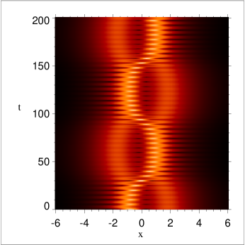
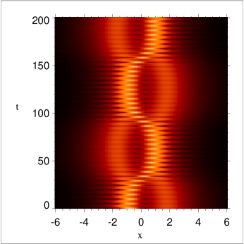
Figure 2: A two-soliton bound state affected by an attractive perturbation. Here, $\epsilon=0.0387$, $m_{1}=0.6$, and $m_{2}=1$. Left: an approximation to $|\psi|^{2}$ found by solving Newton’s equations and then constructing the field using reflectionless inverse theory. Right: the corresponding numerics for (1). The bound state has too much energy for the harmonic approximation to hold, and the period of motion, about $120$ time units, is longer than the harmonic period.

For small displacements, we have $F(q;\tilde{M})=-k(\tilde{M})q+O(q^{2})$. The (mass-dependent) spring constant $k(\tilde{M})$ determines the frequency $\omega(\tilde{M}):=(k(\tilde{M})/\tilde{M})^{1/2}$ of small oscillatory motions. This is the frequency on the time scale $S$; the frequency on the original time scale $t$ is related by $\Omega(m_{1},m_{2},\epsilon)=\epsilon\,(m_{1}m_{2})^{3/2}\omega(\tilde{m}/(m_{1}m_{2})^{1/2})$. A formula for the spring constant $k(\tilde{M})$ can be found by simply differentiating with respect to $q$ in (65) and setting $q=0$, however it seems less useful to present than a plot, shown in Figure 3, of the (numerically) evaluated formula. In Figure 4 we plot the corresponding frequency (on the time scale $S$), the latter being a directly observable quantity.

Figure 3: The spring constant for small bound motions as a function $\tilde{M}$.

Figure 4: The frequency $\omega$ of harmonic motion as a function $\tilde{M}$.

It is noteworthy here that the dynamics of solitons can be described by a linear theory even though their amplitudes are not at all small. The parameter linearizing the theory is the distance between the solitons, rather than the soliton amplitude. We also remark that the limit in which this linear behavior holds is that of infinitessimally-separated solitons, a limit in which methods assuming the solitons to be well-separated are invalid.

4.6 Repulsive case. Asymptotic velocity.

For $\sigma=-1$, the force and displacement $q$ have the same sign, resulting in $q$ always becoming large. Solitons that are near each other at $t=0$ are ejected from the origin as observed by Artigas et. al. [21]. This effect is captured accurately by our theory, as shown in Figure 5.

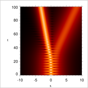
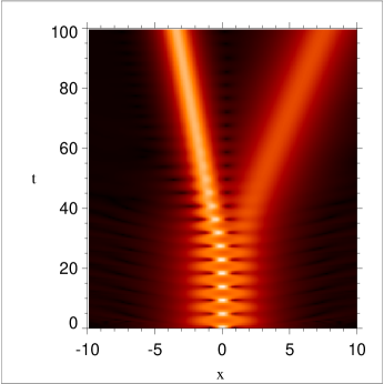
Figure 5: A two-soliton bound state affected by a repulsive perturbation. Here, $\epsilon=0.07746$, $m_{1}=0.4$, and $m_{2}=1$. As in Figure 2, the result of perturbation theory is on the left and the numerics are on the right. The solitons escape with a relative “ejection” velocity given by (68).

The work done by the force in moving the particle from $q=q_{0}$ to $q=\infty$ determines the asymptotic velocity of an initially stationary particle upon ejection. Taking $q_{0}=0$ corresponds to the ultimate velocity of a stationary particle that is slightly perturbed from (unstable) equilibrium at the origin. With zero initial velocity, one equates the asymptotic kinetic energy with the work done:

$$\frac{1}{2}\tilde{M}q^{\prime}(\infty)^{2}=\int_{q_{0}}^{\infty}F(q;\tilde{M})\,dq\,,$$ (67)

to find a formula for the asymptotic velocity difference:

$$q^{\prime}(\infty)=\left(\frac{2}{\tilde{M}}\int_{q_{0}}^{\infty}\int_{-\infty}^{\infty}H(q,z)\,dz\,dq\right)^{1/2}\,.$$ (68)

Figure 6 shows the asymptotic velocity difference $q^{\prime}(\infty)$ for $q_{0}=0$ found from (68) as a function of the normalized effective mass $\tilde{M}$.

Figure 6: The asymptotic velocity difference $q^{\prime}(\infty)$ of two solitons falling from unstable equilibrium.

To apply the graph in Figure 6 to problems with unnormalized masses, it is useful to unravel the changes of variables made so far. Given $m_{1}$ and $m_{2}$, the scaling parameter is $\xi=(m_{1}m_{2})^{-1/2}$ and the effective mass is $\tilde{m}=2\cdot(m_{1}^{-1}+m_{2}^{-1})^{-1}$. Then, the normalized effective mass used in Figure 6 is $\tilde{M}=\xi\tilde{m}$. Next, from the graph one finds the asymptotic velocity $q^{\prime}(\infty)$. The true velocity in the original coordinates is then $dy/dt=\epsilon\xi^{-2}q^{\prime}(\infty)$. For example, the parameters used in Figure 5 imply a normalized effective mass of $\tilde{M}\approx 0.9$. From Figure 6 one finds $q^{\prime}(\infty)\approx 5.0$, and thus $dy/dt\approx 0.15$. This value agrees well with the pictures in Figure 5.

In the attractive case, the integral (67) also has physical meaning as the binding energy of the two-soliton state. A relative velocity in excess of $q^{\prime}(\infty)$, the escape velocity, will “ionize” the state.

5 Discussion

Multiscale asymptotics shows that under certain conditions the behavior of a multisoliton initial condition in a perturbed NLSE reduces to Newton’s equations for a system of interacting particles, one particle per soliton. The theory applies over time scales of length $O(\epsilon^{-1})$ for perturbations of size $\epsilon^{2}$, when the initial velocities of the solitons mutually differ by an $O(\epsilon)$ amount. Our calculations make very concrete the often-cited analogy between solitons and particles. We want to emphasize that the limit considered here is one in which the relative velocities of the solitons are small but the solitons may be strongly nonlinearly superimposed, precisely the limit in which methods exploiting large distances between solitons fail.

For a quintic perturbation of the NLSE and an initial condition composed of two solitons, the resulting dynamical system can be analyzed. When the perturbation is attractive ($\sigma=+1$), the system describes a nonlinear oscillator with all solutions $q(S)$ being periodic. If the energy associated with $q(S)$ is small (that is, if $q(0)$ and $q^{\prime}(0)$ are both small), then the periodic motion is nearly harmonic, and formulae for the associated spring constant and frequency of motion can be found; in this limit the model for the soliton interaction linearizes even though the soliton amplitudes are not at all small. The latter are determined by the masses $m_{1}$ and $m_{2}$ and are not related to the coordinate $q(S)$. For larger energies, the spring “softens” and the frequency decreases with increasing energy. The pictures in Figure 2 show oscillations in the nonlinear regime, where the frequency of motion is smaller than the linear frequency. Of course even in the nonlinear regime, the dynamics still obey the simple model $\tilde{M}q^{\prime\prime}=F(q;\tilde{M})$. Although the periodic motion is predicted and observed over long time scales of size $O(\epsilon^{-1})$, it is not likely to persist for all time, due to the influence of higher-order resonant coupling effects.

On the other hand, when the quintic perturbation is repulsive ($\sigma=-1$), the nodal point at the origin in the phase plane gets replaced with an unstable saddle point. All orbits apart from the fixed point itself represent the nonlinear development of the instability. Because the force vanishes fast enough for large $q$, the velocity $q^{\prime}(S)$ ultimately saturates as the two-soliton state becomes “ionized”. From the force function $F(q;\tilde{M})$ this “ejection” velocity may be calculated, giving excellent agreement with direct simulations of the perturbed NLSE. This analysis explains the observations reported in [21]. The symmetry-breaking that determines which soliton ends up on the right and which on the left can be traced to the location of the initial phase point in relation to the separatrix connected to the saddle. Unlike in the attractive ($\sigma=+1$) case, the approximation obtained from multiscale asymptotics for the repulsive ($\sigma=-1$) case is expected to be uniformly valid for all time, since as the solitons separate, further effects due to resonant coupling diminish.

Given the formula for the force $F(q;\tilde{M})$, it is possible to compute the harmonic frequency and ejection velocity, more explicitly than we have done here. For example, the formulae would be expected to simplify in the limits $\tilde{M}\downarrow 0$ (corresponding to two solitons differing very much in amplitude) and $\tilde{M}\uparrow 1$ (corresponding to two solitons with nearly the same amplitude). The calculation of the ejection velocity is challenging because it may require uniform approximation of $F(q;\tilde{M})$ for all $q$ in the limit of interest; pointwise asymptotics for fixed $q$ are not enough to approximate the work integral without further information.

6 Acknowledgements

PDM acknowledges the support of NSF grant DMS 9304580 while a member of the School of Mathematics at the Institute for Advanced Study. During the preparation of this paper, JAB and NNA were affiliated with the Australian Photonics Cooperative Research Centre.

Appendix: Formulae for the Two-Particle Force Function Integrand

Here, we record the details of the formulae for the two-particle force function needed to calculate or approximate for special values of $\tilde{M}$ the force and related quantities to any desired accuracy.

Before averaging. The thirteen terms appearing in the sum in (57) are given here in terms of $c:=\cos\theta$, $S_{k}:=\sinh(\zeta_{k})$ and $C_{k}:=\cosh(\zeta_{k})$, $\zeta_{1}:=2m_{1}(z+y/2)$ and $\zeta_{2}:=2m_{2}(z-y/2)$.

$$h_{1}=2m_{1}^{6}m_{2}S_{2}C_{1}C_{2}^{6}+2m_{1}m_{2}^{6}S_{1}C_{1}^{6}C_{2}\hskip 21.68121pth_{2}=-\Big{(}m_{1}^{5}(m_{2}^{2}+m_{1}^{2})S_{1}C_{2}^{7}+m_{2}^{5}(m_{2}^{2}+m_{1}^{2})S_{2}C_{1}^{7}\Big{)}$$

$$h_{3}=2m_{1}^{5}(m_{1}^{2}+m_{2}^{2}c^{2})S_{1}C_{2}^{5}+2m_{2}^{5}(m_{1}^{2}c^{2}+m_{2}^{2})S_{2}C_{1}^{5}$$

$$h_{4}=-\Big{(}2m_{1}^{5}(m_{2}^{2}+m_{1}^{2})cS_{2}C_{2}^{5}+2m_{2}^{5}(m_{2}^{2}+m_{1}^{2})cS_{1}C_{1}^{5}\Big{)}$$

$$h_{5}=m_{1}^{5}(m_{1}^{2}-9m_{2}^{2})cS_{2}C_{1}^{2}C_{2}^{5}+m_{2}^{5}(m_{2}^{2}-9m_{1}^{2})cS_{1}C_{1}^{5}C_{2}^{2}$$

$$h_{6}=m_{1}^{4}m_{2}(5m_{2}^{2}+3m_{1}^{2})cS_{1}C_{1}C_{2}^{6}+m_{1}m_{2}^{4}(3m_{2}^{2}+5m_{1}^{2})cS_{2}C_{1}^{6}C_{2}$$

$$h_{7}=-\Big{(}2m_{1}^{4}m_{2}((5m_{1}^{2}+m_{2}^{2})c+4m_{2}^{2}c^{3})S_{1}C_{1}C_{2}^{4}+2m_{1}m_{2}^{4}((m_{1}^{2}+5m_{2}^{2})c+4m_{1}^{2}c^{3})S_{2}C_{1}^{4}C_{2}\Big{)}$$

$$h_{8}=2m_{1}^{4}m_{2}(m_{2}^{2}+(5m_{1}^{2}+4m_{2}^{2})c^{2})S_{2}C_{1}C_{2}^{4}+2m_{1}m_{2}^{4}(m_{1}^{2}+(5m_{2}^{2}+4m_{1}^{2})c^{2})S_{1}C_{1}^{4}C_{2}$$

$$h_{9}=-\Big{(}2m_{1}^{3}m_{2}^{4}(1+4c^{2})S_{1}C_{1}^{2}C_{2}^{5}+2m_{1}^{4}m_{2}^{3}(1+4c^{2})S_{2}C_{1}^{5}C_{2}^{2}\Big{)}$$

$$h_{10}=m_{1}^{4}m_{2}(3m_{2}^{2}-m_{1}^{2})(1+4c^{2})S_{2}C_{1}^{3}C_{2}^{4}+m_{1}m_{2}^{4}(3m_{1}^{2}-m_{2}^{2})(1+4c^{2})S_{1}C_{1}^{4}C_{2}^{3}$$

$$h_{11}=-\Big{(}2m_{1}^{3}m_{2}^{2}(m_{2}^{2}-m_{1}^{2})(3c+2c^{3})S_{2}C_{1}^{4}C_{2}^{3}+2m_{1}^{2}m_{2}^{3}(m_{1}^{2}-m_{2}^{2})(3c+2c^{3})S_{1}C_{1}^{3}C_{2}^{4}\Big{)}$$

$$h_{12}=-\Big{(}4m_{1}^{2}m_{2}^{3}((3m_{1}^{2}+m_{2}^{2})c+(2m_{1}^{2}+4m_{2}^{2})c^{3})S_{1}C_{1}^{3}C_{2}^{2}+4m_{1}^{3}m_{2}^{2}((3m_{2}^{2}+m_{1}^{2})c+(2m_{2}^{2}+4m_{1}^{2})c^{3})S_{2}C_{1}^{2}C_{2}^{3}\Big{)}$$

$$h_{13}=4m_{1}^{2}m_{2}^{3}(m_{2}^{2}+(3m_{1}^{2}+4m_{2}^{2})c^{2}+2m_{1}^{2}c^{4})S_{2}C_{1}^{3}C_{2}^{2}+4m_{1}^{3}m_{2}^{2}(m_{1}^{2}+(3m_{2}^{2}+4m_{1}^{2})c^{2}+2m_{2}^{2}c^{4})S_{1}C_{1}^{2}C_{2}^{3}$$

After normalization and averaging. Here, we give the nonzero quantities $g_{mn}=g_{mn}(\alpha,\beta)$ appearing in (66). In these expressions $\beta$ and $\alpha$ are linked by the normalization condition $\alpha\beta=1$.

$$\begin{array}[]{rclrcl}g_{03}&=&672\alpha^{3}-672\alpha^{7}&g_{04}&=&1344\alpha^{3}+3136\alpha^{7}\\ g_{05}&=&-2304\alpha^{3}-2816\alpha^{7}&g_{06}&=&512\alpha^{3}+512\alpha^{7}\end{array}$$

$$\begin{array}[]{rcl}g_{12}&=&-6048\alpha^{3}-4032\alpha^{7}+10080\beta\\ g_{13}&=&69664\alpha^{3}+16576\alpha^{7}+1120\alpha^{11}+2240\beta\\ g_{14}&=&-130544\alpha^{3}-52016\alpha^{7}-2960\alpha^{11}-29520\beta\\ g_{15}&=&75904\alpha^{3}+48256\alpha^{7}+4480\alpha^{11}+18816\beta\\ g_{16}&=&-10368\alpha^{3}-10368\alpha^{7}-1920\alpha^{11}-1920\beta\end{array}$$

$$\begin{array}[]{rcl}g_{21}&=&-13440\alpha^{3}+3360\beta+10080\beta^{5}\\ g_{22}&=&17920\alpha^{3}+17920\alpha^{7}+51520\beta-24640\beta^{5}\\ g_{23}&=&-234720\alpha^{3}-48320\alpha^{7}-5440\alpha^{11}-272640\beta-7200\beta^{5}\\ g_{24}&=&479872\alpha^{3}+146176\alpha^{7}+13184\alpha^{11}+320\alpha^{15}+352704\beta+36864\beta^{5}\\ g_{25}&=&-277152\alpha^{3}-144096\alpha^{7}-19280\alpha^{11}-560\alpha^{15}-141808\beta-15120\beta^{5}\\ g_{26}&=&31680\alpha^{3}+31680\alpha^{7}+8800\alpha^{11}+480\alpha^{15}+8800\beta+480\beta^{5}\end{array}$$

$$\begin{array}[]{rcl}g_{30}&=&-4032\beta+3360\beta^{5}+672\beta^{9}\\ g_{31}&=&5600\alpha^{3}-90944\beta-32480\beta^{5}-7616\beta^{9}\\ g_{32}&=&131600\alpha^{3}-6720\alpha^{7}+166960\beta+14960\beta^{5}+15760\beta^{9}\\ g_{33}&=&-24576\alpha^{3}-15168\alpha^{7}+3648\alpha^{11}+249088\beta+145344\beta^{5}-1984\beta^{9}\\ g_{34}&=&-375744\alpha^{3}-63840\alpha^{7}-6688\alpha^{11}-480\alpha^{15}-545056\beta-186144\beta^{5}-9888\beta^{9}\\ g_{35}&=&280368\alpha^{3}+108768\alpha^{7}+13712\alpha^{11}+864\alpha^{15}+16\alpha^{19}\\ &&\hskip 21.68121pt+\,227744\beta+54604\beta^{5}+2592\beta^{9}\\ g_{36}&=&-24024\alpha^{3}-24024\alpha^{7}-8008\alpha^{11}-728\alpha^{15}-8\alpha^{19}-8008\beta-728\beta^{5}-8\beta^{9}\end{array}$$

$$\begin{array}[]{rcl}g_{40}&=&-6720\beta-22400\beta^{5}-2240\beta^{9}\\ g_{41}&=&31680\alpha^{3}+216128\beta+162400\beta^{5}+19072\beta^{9}+800\beta^{13}\\ g_{42}&=&-269952\alpha^{3}-18720\alpha^{7}-592576\beta-268928\beta^{5}-29984\beta^{9}-2560\beta^{13}\\ g_{43}&=&384912\alpha^{3}+82032\alpha^{7}+2976\alpha^{11}+387040\beta+43584\beta^{5}-8784\beta^{9}+1168\beta^{13}\\ g_{44}&=&-81312\alpha^{3}-63840\alpha^{7}-8256\alpha^{11}-192\alpha^{15}\\ &&\hskip 21.68121pt+\,97152\beta+127104\beta^{5}+26784\beta^{9}+864\beta^{13}\\ g_{45}&=&-61776\alpha^{3}+4368\alpha^{11}+288\alpha^{15}-96096\beta-39312\beta^{5}-4032\beta^{9}-48\beta^{13}\end{array}$$

$$\begin{array}[]{rcl}g_{50}&=&9216\beta+21760\beta^{5}+4864\beta^{9}\\ g_{51}&=&-20096\alpha^{3}-129152\beta-155264\beta^{5}-38272\beta^{9}-1280\beta^{13}\\ g_{52}&=&112848\alpha^{3}+7584\alpha^{7}+355920\beta+307872\beta^{5}+71872\beta^{9}+3984\beta^{13}+80\beta^{17}\\ g_{53}&=&-165584\alpha^{3}-22752\alpha^{7}-528\alpha^{11}\\ &&\hskip 21.68121pt-\,330528\beta-200112\beta^{5}-32672\beta^{9}-1392\beta^{13}-96\beta^{17}\\ g_{54}&=&72072\alpha^{3}+15288\alpha^{7}+648\alpha^{11}\\ &&\hskip 21.68121pt+\,92664\beta+24024\beta^{5}-6552\beta^{9}-1512\beta^{13}-24\beta^{17}\end{array}$$

$$\begin{array}[]{rcl}g_{60}&=&-1536\beta-4096\beta^{5}-1536\beta^{9}\\ g_{61}&=&1280\alpha^{3}+13568\beta+27648\beta^{5}+13568\beta^{9}+1280\beta^{13}\\ g_{62}&=&-4096\alpha^{3}-96\alpha^{7}-27808\beta-50688\beta^{5}-27808\beta^{9}-4096\beta^{13}-96\beta^{17}\\ g_{63}&=&2912\alpha^{3}+112\alpha^{7}+16016\beta+27456\beta^{5}+16016\beta^{9}+2912\beta^{13}+112\beta^{17}\end{array}$$

References

• [1] V. E. Zakharov and A. V. Shabat, “Exact theory of two-dimensional self-focusing and one-dimensional self modulation of waves in nonlinear media”, Sov. Phys. JETP, 34, 62–68, 1972. (in Russian as Zh. Eksp. Teor. Fiz., 61, 118–134, 1971.)
• [2] N. N. Akhmediev and A. Ankiewicz, Solitons : Nonlinear Pulses and Beams, Chapman and Hall, New York, 1997.
• [3] A. Hasegawa and F. Tappert, “Transmission of stationary nonlinear optical pulses in dispersive dielectric fibers, I. Anomalous dispersion”, App. Phys. Lett., 23, 142–144, 1973.
• [4] A. Hasegawa and F. Tappert, “Transmission of stationary nonlinear optical pulses in dispersive dielectric fibers, II. Normal dispersion”, App. Phys. Lett., 23, 171–172, 1973.
• [5] G. P. Agrawal, Nonlinear Fiber Optics, Academic Press, New York, 1989.
• [6] A. Hasegawa and Y. Kodama, Solitons in Optical Communications, Clarendon Press, Oxford, 1995.
• [7] V. I. Karpman and E. M. Maslov, “Perturbation theory for solitons”, Zh. Eksp. Teor. Fiz. (JETP), 46, 281–291, 1977.
• [8] G. L. Lamb, Elements of Soliton Theory, Wiley Interscience, New York, 1980.
• [9] J. P. Gordon, “Interaction forces among solitons in optical fibers”, Opt. Lett., 8, 596–598, 1983.
• [10] C. Desem and P. L. Chu, “Reducing soliton interaction in single-mode optical fibres”, IEE Proc. J, 134, 145–150, 1987.
• [11] A. Ankiewicz, “Simplified description of soliton perturbation and interaction using averaged complex potentials”, J. Nonlin. Opt. Phys. and Mat., 4, 857–870, 1995.
• [12] C. Desem and P. L. Chu, “Soliton interaction in the presence of loss and periodic amplification in optical fibres”, Opt. Lett., 12, 349–351, 1987.
• [13] C. Desem and P. L. Chu, “Soliton interaction in the presence of source chirping and mutual interaction in single-mode optical fibres”, Elec. Lett., 23, 260–262, 1987.
• [14] A. D. Boardman, H. M. Mehta, A. K. Sangarpaul, and K. Xie, “Interactions of bright $N$-soliton trains propagating in birefringent optical fibres”, Opt. Comm., 116, 208–218, 1995.
• [15] D. J. Kaup and A. C. Newell, “Solitons as particles, oscillators, and in slowly changing media: A singular perturbation theory”, Proc. Roy. Soc. Lond. A, 361, 413–446, 1978.
• [16] D. Anderson, “Variational approach applied to nonlinear pulse propagation in optical fibres”, Phys. Rev. A., 27, 3135–3145, 1983.
• [17] G. B. Whitham, Linear and Nonlinear Waves, Wiley Interscience, New York, 1974.
• [18] A. B. Aceves, J. V. Moloney, and A. C. Newell, “Theory of light-beam propagation at nonlinear interfaces, II. Multiple-particle and multiple-interface extensions”, Phys. Rev. A, 39, 1809–1827, 1989.
• [19] A. B. Aceves, P. Varatharajah, A. C. Newell, E. M. Wright, G. I. Stegeman, D. R. Heathley, J. V. Moloney, and H. Adachihara, “Particle aspects of collimated light channel propagation at nonlinear interfaces and in waveguides”, J. Opt. Soc. Am. B, 7, 963–974, 1990.
• [20] A. V. Buryak and N. N. Akhmediev, “Internal friction between solitons in near-integrable systems” Phys. Rev. E, 50, 3126–3133, 1994.
• [21] D. Artigas, L. Torner, J. P. Torres, and N. N. Akhmediev, “Asymmetrical splitting of higher-order optical solitons induced by quintic nonlinearity”, Opt. Comm., 143, 322–328, 1997.
• [22] J. A. Besley, P. D. Miller, and N. N. Akhmediev, “Linear guidance properties of solitonic Y-junction waveguides”, Opt. Quant. Elect., to appear, 2000.
• [23] L. D. Faddeev and L. A. Takhtajan, Hamiltonian Methods in the Theory of Solitons, Springer Verlag, Berlin, 1987.
• [24] J. A. Besley, Modes and Solitons in Waveguide Optics, PhD thesis, The Australian National University, Canberra, 1998.
• [25] I. M. Krichever, “Integration of nonlinear equations by methods of algebraic geometry”, Funkts. Anal. Pril., 9, 77–78, 1975.
• [26] Yu. I. Manin, “Aspects of nonlinear differential equations”, J. Sov. Math., 11, 1979.
• [27] E. Date, “Multi-soliton solutions and quasi-periodic solutions of nonlinear equations of Sine-Gordon type”, Osaka J. Math., 19, 125–158, 1982.
• [28] P. D. Miller and N. N. Akhmediev, “Transfer matrices for multiport devices made from solitons”, Phys. Rev. E, 76, 4098–4106, 1996.