Instabilities of Hexagonal Patterns with Broken Chiral Symmetry

Abstract

Three coupled Ginzburg-Landau equations for hexagonal patterns with broken chiral symmetry are investigated. They are relevant for the dynamics close to onset of rotating non-Boussinesq or surface-tension-driven convection. Steady and oscillatory, long- and short-wave instabilities of the hexagons are found. For the long-wave behavior coupled phase equations are derived. Numerical simulations of the Ginzburg-Landau equations indicate bistability between spatio-temporally chaotic patterns and stable steady hexagons. The chaotic state can, however, not be described properly with the Ginzburg-Landau equations.

PACS: 47.54.+r,47.27.Te, 47.20.Dr, 47.20.Ky

Keywords: Hexagon Patterns, Rotating Convection, Ginzburg-Landau Equation, Phase Equation, Sideband Instabilities, Spatiotemporal Chaos

I Introduction

Convection has played a key role in the elucidation of the spatio-temporal dynamics arising in nonequilibrium pattern forming systems. The interplay of well-controlled experiments with analytical and numerical theoretical work has contributed to a better understanding of various mechanisms that can lead to complex behavior. From a theoretical point of view the effect of rotation on roll convection has been particularly interesting because it can lead to spatio-temporal chaos immediately above threshold where the small amplitude of the pattern allows a simplified treatment. Early work of Küppers and Lortz [1, 2] showed that for sufficiently large rotation rate the roll pattern becomes unstable to another set of rolls rotated with respect to the initial one. Due to isotropy the new set of rolls is also unstable and persistent dynamics are expected. Later Busse and Heikes [3] confirmed experimentally the existence of this instability and the persistent dynamics arising from it. They proposed an idealized model of three coupled amplitude equations in which the instability leads to a heteroclinic cycle connecting three sets of rolls rotated by 120^o with respect to each other. Recently the Küppers-Lortz instability and the ensuing dynamics have been subject to intensive research, both experimentally [4, 5, 6, 7, 8] and theoretically [9, 10, 11, 12, 13, 14, 15]. It is found that in sufficiently large systems the switching between rolls of different orientation looses coherence and the pattern breaks up into patches in which the rolls change orientation at different times. The shape and size of the patches changes persistently due to the motion of the fronts separating them. Other interesting aspects induced by rotation are the modification of the dynamics of defects [16] and an unexpected transition to square patterns [17].

In this paper we are interested in the effect of rotation on hexagonal rather than roll (stripe) patterns as they arise in systems with broken up-down symmetry (e.g. non-Boussines convection or surface-tension driven convection). Complex dynamics, if they are indeed induced by the rotation, are likely to differ qualitatively from those in roll patterns due to the difference in the symmetry of the pattern. Considering the small-amplitude regime close to onset, we use coupled Ginzburg-Landau equations. On this level the Coriolis force arising from rotation manifests itself as a breaking of the chiral symmetry. We therefore consider quite generally the effect of chiral symmetry breaking on weakly nonlinear hexagonal patterns. Since the equations are derived from the symmetries of the system we expect them to capture the generic behavior close to onset.

The dynamics of strictly periodic hexagon patterns with broken chiral symmetry have been investigated in detail by Swift [18] and Soward [19]. They found that the heteroclinic orbit of the Busse-Heikes model is replaced by a periodic orbit arising from a secondary Hopf bifurcation off the hexagons. Their results have been confirmed in numerical simulations of a Swift-Hohenberg-type model [20]. The competition between hexagons, rolls, and squares in rotating Bénard-Marangoni convection has been considered in [21]. In the present paper we focus on the impact of rotation on the side-band instabilities of steady hexagon patterns, i.e. on instabilities that introduce modes with wavelengths or orientation different than those of the hexagons themselves. Thus, we extend the work of Sushchik and Tsimring [22] to the case of broken chiral symmetry. We find that rotation can increase the wavenumber range over which the hexagons are stable with respect to long-wave perturbations. For larger values of the control parameter, however, additional short-wave instabilities arise. The long- and the short-wave modes can be steady or oscillatory. While in most cases they eventually lead to stable hexagon or roll patterns with different wavevectors, they can also induce persistent dynamics that can apparently not be described with Ginzburg-Landau equations.

The paper is organized as follows. In the following section we use symmetry arguments to introduce the appropriate Ginzburg-Landau equations. The stability with respect to long-wave perturbations is addressed in section III in which the coupled phase equations for the system are derived. General perturbations (within the Ginzburg-Landau framework) are considered in section IV. In section V we investigate numerically the nonlinear behavior resulting from the side-band instabilities. Conclusions are given in section VI.

II Amplitude equations

We consider small-amplitude hexagon patterns in systems with broken chiral symmetry. For strictly periodic patterns the amplitudes ${\cal A}_{i}$ of the three sets of rolls (stripes) that make up the hexagon satisfy then the equations [23]

$$\partial_{t}{\cal A}_{1}=\epsilon{\cal A}_{1}+\alpha_{0}\overline{\cal A}_{2}\overline{\cal A}_{3}-g_{1}{\cal A}_{1}|{\cal A}_{1}|^{2}-g_{2}{\cal A}_{1}|{\cal A}_{2}|^{2}-g_{3}{\cal A}_{1}|{\cal A}_{3}|^{2},$$ (1)

where the equations for the other two amplitudes are obtained by cyclic permutation of the indices and $\epsilon$ is a small parameter related to the distance from threshold. The overbar represents complex conjugation. These equations can be obtained from the corresponding physical equations (e.g. Navier-Stokes) using a perturbative technique with the usual scalings (${\cal A}\sim{\mathcal{O}}(\epsilon^{1/2})$ and $\partial_{t}\sim{\mathcal{O}}(\epsilon)$). In order for all terms in (1) to be of the same order the coefficient of the quadratic term must be small, $\alpha_{0}\sim{\mathcal{O}}(\epsilon^{1/2})$. This term arises from a resonance of the wavevectors of the three modes in the plane. The broken chiral symmetry manifests itself by the cross-coupling coefficients not being equal, $g_{2}\neq g_{3}$.

For completeness it should be noted that rotation leads in convection not only to a chiral symmetry breaking but also to a (weak) breaking of the translation symmetry due to the centrifugal force. In the following we will consider it to be negligible. In addition, for sufficiently small Prandtl number rotation can render the primary instability oscillatory [24, 13].

In order to analyze the possibility of modulational instabilities spatial derivatives must be included in Eq. (1). We take the gradients in both directions to be of the same order, $\nabla\sim{\mathcal{O}}(\epsilon^{1/2})$ [25], and retain both linear and quadratic gradient terms. After rescaling the amplitude, time, and space we arrive at the equations,

$$\partial_{t}A_{1} = \mu A_{1}+({\bf{n}}_{1}\cdot\nabla)^{2}A_{1}+\overline{A}_{2}\overline{A}_{3}-A_{1}|A_{1}|^{2}-(\nu+\tilde{\nu})A_{1}|A_{2}|^{2}-(\nu-\tilde{\nu})A_{1}|A_{3}|^{2}$$ (4)

$$+i(\alpha_{1}+\tilde{\alpha})\overline{A}_{2}({\bf{n}}_{3}\cdot\nabla)\overline{A}_{3}+i(\alpha_{1}-\tilde{\alpha})\overline{A}_{3}({\bf{n}}_{2}\cdot\nabla)\overline{A}_{2}$$

$$+i\alpha_{2}\left(\overline{A}_{2}(\mbox{\boldmath$\tau$}_{3}\cdot\nabla)\overline{A}_{3}-\overline{A}_{3}(\mbox{\boldmath$\tau$}_{2}\cdot\nabla)\overline{A}_{2}\right)$$

where now all the coefficients are ${\cal O}(1)$, and ${\bf n}_{i}$ and $\mbox{\boldmath$\tau$}_{i}$ represent the unit vectors parallel and perpendicular to the wavenumber ${\bf k}_{i}$ (Fig. 1). The cross-coupling coefficients have been rewritten in terms of $\nu$ and $\tilde{\nu}$, with $\tilde{\nu}$ being proportional to rotation and therefore giving a measure of the chiral symmetry breaking. In the gradient terms the chiral symmetry breaking manifests itself in the terms proportional to $\tilde{\alpha}$.

FIG. 1.: a) Critical wavenumbers ${\bf k}_{1},{\bf k}_{2},{\bf k}_{3}$. They satisfy the relation ${\bf k}_{1}+{\bf k}_{2}+{\bf k}_{3}=0$. Up to a global rotation $\Psi$, the position of the wavevectors is given by the modulus of two of them and the angle between them. The symbols ${\bf n}_{i}$ and $\mbox{\boldmath$\tau$}_{i}$ denote the unit vectors in the parallel and perpendicular directions to the wavevectors, respectively. b) The replacement $A_{i}\rightarrow A_{i}e^{iK{\bf n}_{i}}$ represents a change in the magnitude of the wavevector while $A_{i}\rightarrow A_{i}e^{iK\mbox{\boldmath$\tau$}_{i}}$ represents a rotation of it.

The influence of the nonlinear gradient terms in (4) involving $\alpha_{1}$ and $\alpha_{2}$ has been studied by several authors [26, 27, 28]. The origin of the new term involving $\tilde{\alpha}$ is best understood by considering the coefficient $\alpha$ of the quadratic term. The gradient terms arise from its dependence on the wavenumber of the modes involved, $\alpha=\alpha({\bf{k}}_{1},{\bf{k}}_{2},{\bf{k}}_{3})$ i.e. when the equation is considered in Fourier space. Due to the resonance condition (${\bf{k}}_{1}+{\bf{k}}_{2}+{\bf{k}}_{3}=0$) we can drop the dependence on one of the wavevectors. Then, up to an arbitrary global rotation $\Psi$, the system can be specified by the angle $\Theta$ between the wavevectors ${\bf k}_{2}$ and ${\bf k}_{3}$ and their moduli $k_{2}$ and $k_{3}$ (see Fig. 1). Due to isotropy the coefficient $\alpha$ cannot depend on the global rotation and can therefore be expressed as $\alpha=\alpha(k_{2},k_{3},\Theta)$. When evaluated at the critical values of the wavenumbers $\alpha_{0}$ is given by $\alpha_{0}=\alpha(k^{c}_{2},k^{c}_{3},\Theta^{c}=2\pi/3)$ (in Eq. (4) we take the normalization $\alpha_{0}=1$). Since a change in the modulus of ${\bf k}_{i}$ can be effected by the replacement $A_{i}\rightarrow A_{i}e^{iK{\bf n}_{i}}$ the dependence of $\alpha$ on the moduli $k_{2}$ and $k_{3}$ can be represented in real space by

$$\frac{\partial\alpha}{\partial k_{2}}\overline{A}_{3}({\bf{n}}_{2}\cdot\nabla)\overline{A}_{2}+\frac{\partial\alpha}{\partial k_{3}}\overline{A}_{2}({\bf{n}}_{3}\cdot\nabla)\overline{A}_{3}.$$ (5)

When the chiral symmetry is broken $\partial\alpha/\partial k_{2}$ and $\partial\alpha/\partial k_{3}$ need not be equal and it is convenient to introduce the coefficients

$$\alpha_{1}=\frac{1}{2}\left(\frac{\partial\alpha}{\partial k_{3}}+\frac{\partial\alpha}{\partial k_{2}}\right)\makebox[28.45274pt]{and}\tilde{\alpha}=\frac{1}{2}\left(\frac{\partial\alpha}{\partial k_{3}}-\frac{\partial\alpha}{\partial k_{2}}\right)$$ (6)

with $\alpha_{1}$ even and $\tilde{\alpha}$ odd in the amplitude of the symmetry breaking.

On the other hand, a variation in the angle between ${\bf{k}}_{2}$ and ${\bf{k}}_{3}$ is represented by

$$\frac{i}{k_{c}}\frac{\partial\alpha}{\partial\Theta}(\overline{A}_{2}(\mbox{\boldmath$\tau$}_{3}\cdot\nabla)\overline{A}_{3}-\overline{A}_{3}(\mbox{\boldmath$\tau$}_{2}\cdot\nabla)\overline{A}_{2})$$ (7)

with only one coefficient $\alpha_{2}=(\partial\alpha/\partial\Theta)/k_{c}$. This term is invariant under reflections interchanging modes $A_{2}$ and $A_{3}$, since in contrast to the normal vector ${\bf n}_{i}$ the tangential vector $\mbox{\boldmath$\tau$}_{i}$ changes sign in this reflection. Therefore the coefficient $\alpha_{2}$ is even in the amplitude of the symmetry breaking.

Equation (4) admits hexagon solutions $A_{i}=He^{iK\hat{\bf n}_{i}\cdot{\bf{x}}+i\phi_{i}}$ with a sligthly offcritical wavenumber (${\bf k}_{i}={\bf k}^{c}_{i}+{\bf K}_{i}$, $K\ll k_{c}$), with

$$H=\frac{(1+2K\alpha_{1})\pm\sqrt{(1+2K\alpha_{1})^{2}+4(\mu-K^{2})(1+2\nu)}}{2(1+2\nu)},\qquad\Phi\equiv\phi_{1}+\phi_{2}+\phi_{3}=0.$$ (8)

The stability of this solution to perturbations with the same wavevectors has been studied by several authors [18, 19] and can be summarized in the bifurcation diagram shown in Fig. 2. The hexagons appear through a saddle-node bifurcation at $\mu=\mu_{sn}$,

$$\mu_{sn}=-\frac{(1+2K\alpha_{1})^{2}}{4(1+2\nu)}+K^{2},$$ (9)

and become unstable $via$ a Hopf bifurcation at $\mu=\mu_{H}$,

$$\mu_{H}=\frac{(1+2K\alpha_{1})^{2}(2+\nu)}{(\nu-1)^{2}}+K^{2},$$ (10)

with a critical frequency $\omega_{c}=2\sqrt{3}\tilde{\nu}(1+2K\alpha_{1})^{2}/(\nu-1)^{2}$. Note that the Hopf frequency does not depend on $\tilde{\alpha}$. The Hopf bifurcation is supercritical and for $\mu>\mu_{H}$ stable oscillations in the three amplitudes of the hexagonal pattern arise with a phase shift of $2\pi/3$ between them [18, 19, 20], resulting in what we are going to call oscillating hexagons. As $\mu$ is increased further, eventually a point $\mu=\mu_{het}$ is reached at which the branch of oscillating hexagons ends on the branch corresponding to the mixed-mode solution in a global bifurcation involving a heteroclinic connection. Above this point the only stable solution is the roll solution whose stability region is bounded below by

$$\mu_{R}=\frac{1}{(\nu+\tilde{\nu}-1)(\nu-\tilde{\nu}-1)}+K^{2}.$$ (11)

When $|\tilde{\nu}|>\nu-1$ the rolls are never stable and the limit cycle persists for arbitrary large values of $\mu$. In the absence of the quadratic terms in Eq. (1) this condition corresponds to the Küppers-Lortz instability of rolls.

FIG. 2.: Sketch of a bifurcation diagram for a fixed value of the wavenumber $K$.

III Long-Wave approximation: Phase equation

Already below the Hopf bifurcation to oscillating hexagons the hexagonal pattern can be unstable to side-band perturbations. The behavior of long-wavelength modulations is described by the dynamics of the phase of the periodic structure. The phases $\phi_{i}$ of the three modes of the hexagonal pattern can be combined to define a phase vector $\mbox{\boldmath$\phi$}\equiv(\phi_{x},\phi_{y})$, the components $\phi_{x}\equiv-(\phi_{2}+\phi_{3})$ and $\phi_{y}\equiv(\phi_{2}-\phi_{3})/\sqrt{3}$ of which are related to the translation modes in the $x$ - and the $y$ -direction. In the chirally symmetric case the phase vector satisfies the coupled diffusion equations [29, 30]

$$\tau_{0}\partial_{t}\mbox{\boldmath$\phi$ }=D_{\bot}\nabla^{2}\mbox{\boldmath$\phi$ }+(D_{\|}-D_{\bot})\nabla(\nabla\cdot\mbox{\boldmath$\phi$}),$$ (12)

and can be decomposed into a longitudinal (irrotational) and a transversal (divergence free) part $\mbox{\boldmath$\phi$}\equiv\nabla\psi_{l}+\nabla\times\hat{\bf e}_{z}\psi_{t}$. The fields $\psi_{l,t}$ each satisfy a diffusion equation with diffusion constants $D_{\|}$ and $D_{\bot}$, respectively.

We can use symmetry arguments to derive the form of the phase equation when the chiral symmetry is broken. We consider a general diffusion coefficient which is a tensor of rank four,

$$\partial_{t}\phi_{i}=D_{i}^{jkl}\partial_{j}\partial_{k}\phi_{l}$$ (13)

with summation over repeated indices implied. Invariance under reflection and rotations of $60^{o}$ restrict the number of possible independent coefficients $D_{i}^{jkl}$. In the case of broken chiral symmetry we split the diffusion tensor into two parts: one even under reflections, the other odd,

$$D_{i}^{jkl}=\overline{D}_{i}^{jkl}+\Omega_{i}^{m}\tilde{D}_{m}^{jkl},$$ (14)

where $\Omega_{i}^{m}$ is the antisymmetric tensor of rank two given by

$$\Omega=\left(\begin{array}[]{cc}0&-\omega\\ \omega&0\end{array}\right),$$ (15)

with $\omega$ giving the strength of the chiral symmetry breaking (e.g. the rotation frequency). $\bar{D}$ and $\tilde{D}$ are even functions of $\omega$. As generators of the symmetry group we can take rotations of $60^{o}$ and reflections in $x$,

$$R_{60}=\left(\begin{array}[]{cc}\frac{1}{2}&\frac{\sqrt{3}}{2}\\ -\frac{\sqrt{3}}{2}&\frac{1}{2}\end{array}\right),\;\;\kappa_{x}=\left(\begin{array}[]{cc}-1&0\\ 0&1\end{array}\right).$$ (16)

Requiring that $\bar{D}$ and $\tilde{D}$ are invariant under the operations (16) one can show that the most general form of the phase equation with broken quiral symmetry is given by

$$\partial_{t}\mbox{\boldmath$\phi$}=D_{\bot}\nabla^{2}\mbox{\boldmath$\phi$}+(D_{\|}-D_{\bot})\nabla(\nabla\cdot\mbox{\boldmath$\phi$})-D_{\times_{1}}(\hat{\bf e}_{z}\times\nabla^{2}\mbox{\boldmath$\phi$})+D_{\times_{2}}(\hat{\bf e}_{z}\times\nabla)(\nabla\cdot\mbox{\boldmath$\phi$}),$$ (17)

where $\hat{\bf e}_{z}$ is a unit vector in the direction perpendicular to the plane.

It is worth emphasizing that, although the coefficients of this equation can be derived from the amplitude equations, its form is given by symmetry arguments and is, therefore, generic and valid even far from threshold. To derive the phase equation from the amplitude equations (4) we consider a perfect hexagonal pattern with a wavenumber slightly different from critical ($k=k_{c}+K$) and perturb it, both in amplitude and phase, $A_{i}=(H+r_{i})e^{iK\hat{\bf n}_{i}\cdot{\bf{x}}+i\phi_{i}}$. Away from threshold, from the saddle-node and the Hopf bifurcation, the amplitude modes $r_{1},r_{2},r_{3}$, and the global phase $\Phi=\phi_{1}+\phi_{2}+\phi_{3}$ are strongly damped and can be eliminated adiabatically. Following the usual procedures (e.g. [31]) we arrive at Eq. (17) with

$$D_{\bot} = \frac{1}{4}+\frac{1}{u^{2}+\omega^{2}}\left\{\frac{1}{4}H^{2}u[(\alpha_{1}+\sqrt{3}\alpha_{2})^{2}+3\tilde{\alpha}^{2}]-\sqrt{3}H\omega\tilde{\alpha}K-uK^{2}\right\},$$ (18)

$$D_{\|} = D_{\bot}+\frac{1}{2}-\frac{1}{v}\left\{H^{2}\alpha_{1}(\alpha_{1}-\sqrt{3}\alpha_{2})-H(3\alpha_{1}-\sqrt{3}\alpha_{2})K+2K^{2}\right\},$$ (19)

$$D_{\times_{1}} = \frac{1}{u^{2}+\omega^{2}}\left\{\frac{1}{4}\omega H^{2}[(\alpha_{1}+\sqrt{3}\alpha_{2})^{2}+3\tilde{\alpha}^{2}]+\sqrt{3}Hu\tilde{\alpha}K-\omega K^{2}\right\},$$ (20)

$$D_{\times_{2}} = \frac{\tilde{\alpha}}{v}\left\{\sqrt{3}H^{2}\alpha_{1}-\sqrt{3}HK\right\}.$$ (21)

where

$$\omega=2\sqrt{3}H^{2}\tilde{\nu},$$ (22)

$$u=2H^{2}(1-\nu)+2(1+2K\alpha_{1})H,$$ (23)

$$v=2H^{2}(1+2\nu)-(1+2K\alpha_{1})H.$$ (24)

The coefficients $D_{\times_{1}}$ and $D_{\times_{2}}$ are odd in the symmetry-breaking terms $\tilde{\nu}$ and $\tilde{\alpha}$. At the Hopf bifurcation curve $u=0$ implying $H=(1+2K\alpha_{1})/(\nu-1)$ and $\omega=\omega_{c}$, while $v=0$ represents the saddle-node instability.

Expanding the phase in normal modes $\mbox{\boldmath$\phi$}=\mbox{\boldmath$\phi$}^{0}e^{i{\bf{Q}}\cdot{\bf{x}}+\sigma t}$ we obtain the dispersion relation

$$\sigma^{2}+(D_{\|}+D_{\bot})Q^{2}\sigma+\left(D_{\|}D_{\bot}+D_{\times_{1}}(D_{\times_{1}}+D_{\times_{2}})\right)Q^{4}=0,$$ (25)

whose eigenvalues are

$$\sigma_{1,2}=-\frac{1}{2}\left[D_{\|}+D_{\bot}\pm\sqrt{(D_{\|}-D_{\bot})^{2}-4D_{\times_{1}}(D_{\times_{1}}+D_{\times_{2}})}\right]Q^{2}.$$ (26)

When $D_{\times_{1}}=0$ the eigenvalues become simply $\sigma_{1}=-D_{\|}Q^{2}$ and $\sigma_{2}=-D_{\bot}Q^{2}$, corresponding to the eigenvalues of the irrotational and the divergence-free phase modes, respectively. If the rotation rate is small ($D_{\times_{1}},D_{\times_{2}}\ll D_{\bot},D_{\|}$) we can expand (26) and obtain,

$$\sigma_{1}=-\left(D_{\|}-\frac{D_{\times_{1}}(D_{\times_{1}}+D_{\times_{2}})}{(D_{\|}-D_{\bot})}\right)Q^{2},\qquad\sigma_{2}=-\left(D_{\bot}+\frac{D_{\times_{1}}(D_{\times_{1}}+D_{\times_{2}})}{(D_{\|}-D_{\bot})}\right)Q^{2}.$$ (27)

For $D_{\times_{1}},D_{\times_{2}}\sim D_{\|},D_{\bot}$ this approximation is not valid and the longitudinal and transverse perturbations become coupled. An important novelty in this case is that the phase instability can become oscillatory. It occurs when the following conditions are satisfied,

$$D_{\|}+D_{\bot}=0,$$ (28)

$$(D_{\|}-D_{\bot})^{2}-4D_{\times_{1}}(D_{\times_{1}}+D_{\times_{2}})=0.$$ (29)

In Fig. 3 and Fig. 5 (below) we represent the phase instability curves for a number of cases. For small values of the rotation rate $\tilde{\nu}$, the phase stability diagram is similar to that obtained in the absence of rotation, especially for small $\mu$. As $|K|$ is increased, both real eigenvalues in (26) go through zero consecutively as indicated by the dashed and solid lines in Fig.3. As $\mu$ is increased towards the Hopf bifurcation ($\mu\rightarrow\mu_{H}$) the two lines merge and the phase instability becomes oscillatory as indicated by the solid lines. Note that, in contrast to the chirally symmetric case, the left and right stability limits do not merge at $K=0$ as the transition to oscillating hexagons is reached. Instead, they are open and over a range of wavenumbers the hexagons remain stable with respect to long-wave perturbations all the way to the Hopf bifurcation at $\mu=\mu_{H}$. Furthermore, while in the chirally symmetric case the analog of the Hopf bifurcation is transcritical (and steady) and leads discontinously to rolls, the Hopf bifurcation is supercritical and leads to oscillating hexagons [18, 19, 20].

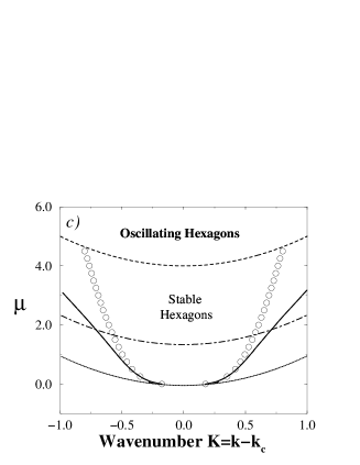
FIG. 3.: Stability diagrams for $\nu=2$, $\tilde{\alpha}=\alpha_{1}=\alpha_{2}=0$ and a) $\tilde{\nu}=0.05$, b) $\tilde{\nu}=0.2$ and c) $\tilde{\nu}=0.5$. The dotted and short-dashed lines indicate the saddle-node and the Hopf bifurcation to oscillating hexagons, respectively. The solid and dashed lines correspond to the long-wave instabilities, while the open circles are the results from the general stability analysis. Rolls are stable with respect to hexagons above the dot-dashed line.

IV General Stability Analysis

We now consider arbitrary perturbations of the hexagonal pattern $A_{i}=(H+a_{i}e^{i{\bf{Q}}\cdot{\bf{x}}+\sigma t})e^{iK\hat{\bf n}_{i}\cdot{\bf{x}}}$, with $a_{1}$, $a_{2}$, $a_{3}$ complex and solve the resulting $6\times 6$ linearized system. Two of the six eigenvalues correspond to the global phase $\Phi$ and the overall amplitude involved in the saddle-node bifurcation. In the regime of interest both are strongly negative. The next two correspond to the translation modes, and can be real or complex. It turns out that these modes can destabilize the hexagons not only via the longwave instabilities (26) but also via short-wave instabilities as illustrated in Fig. 4a, where the solid and dashed lines correspond to the real parts of the complex and real eigenvalues, respectively. Finally, there is a pair of complex conjugate eigenvalues corresponding to the Hopf bifurcation to oscillating hexagons. For some parameter values these eigenvalues merge with the ones corresponding to the phase modes and their real parts become positive (Fig. 4b and 4c). Note that in the chirally symmetric case the eigenvalues are always real and the instabilities long-wave [22].

FIG. 4.: Growth rates (with $\nu=2$, $\tilde{\nu}=0.1$, $\alpha_{1}=\alpha_{2}=0$) when a) the translation modes are short-wave unstable ($\tilde{\alpha}=0$ and $\mu=2.54$, $q=0.53$). The Hopf modes interact with the translation modes and their eigenvalues become positive at finite wavenumber ($\tilde{\alpha}=0.4$): b) Just below the branch switching ($\mu=3.49$, $q=-0.6$), and c) when the Hopf mode is unstable ($\mu=3.75$, $q=-0.57$). The solid and dashed lines correspond to complex and real eigenvalues. The points at which these dispersion relations are obtained are marked by an asterisk in Figs. 3 and 5.

In what follows we will consider $\alpha_{1}=\alpha_{2}=0$ for simplicity. Although non-zero values for these coefficients change the stability boundaries quantitatively, they are not found to induce any qualitatively different instability.

In Figs. 3 and 5 we present the stability limits obtained for several values of $\tilde{\nu}$ and $\tilde{\alpha}$. The short-dashed and the dotted lines correspond to the Hopf and saddle-node bifurcations, respectively, while the dot-dashed line is the curve above which the rolls become stable with respect to the hexagons. We do not address their side-band instabilities. The circles correspond to the results of the general stability analysis while the solid and dashed lines are the stability limits in the long-wave approximation, as given by (26) (with eigenvalues either real or a complex conjugate pair). The solid circles in Fig. 5 correspond to instabilities at finite wavenumber due to the Hopf modes.

Fig. 3 shows the stability limits for $\tilde{\alpha}=0$ but $\tilde{\nu}\neq 0$, i.e. the chiral symmetry is only broken at cubic order. While for small values of the control parameter the long-wave analysis gives the correct stability limits, for larger $\mu$ a steady short-wave instability preempts the long-wave instability before it becomes oscillatory. In this case the eigenvalues are complex for $Q\rightarrow 0$, but they split into two real eigenvalues for larger $Q$, one of which becomes positive (Fig. 4a). As the coefficient $\tilde{\nu}$ is increased the region in which the long-wave instability is relevant decreases (Fig. 3b) and shrinks to almost zero (Fig. 3c).

When the quadratic gradient terms are different from zero the instability regions become asymmetric with respect to $K=0$. The system is, however, invariant under the change $\tilde{\alpha}\rightarrow-\tilde{\alpha}$, $K\rightarrow-K$, $\alpha_{i}\rightarrow-\alpha_{i}$, and we will therefore consider only positive values of $\tilde{\alpha}$. For small $\tilde{\alpha}$ the region of the steady long-wave instability becomes smaller at one side of the bandcenter and larger at the other (Fig. 5a). As $\tilde{\alpha}$ is increased, this region shrinks to zero for $K<0$ and disappears above the Hopf curve for $K>0$. At this point all the instabilities are oscillatory (Fig. 5c). For $\tilde{\alpha}=0.4$ and $\tilde{\alpha}=0.7$ (Fig. 5b,c) the stability limit is entirely given by the longwave results for $K>0$, but for still larger values of $\tilde{\alpha}$ it becomes shortwavelength (Fig. 5d). For $K<0$ there is a large region in which the instability is short-wave and oscillatory. Close to the Hopf bifurcation the instability switches from the translation modes to the Hopf mode (cf. Fig. 4). As $\tilde{\alpha}$ is increased the region in which the instability is due to the Hopf modes grows.

FIG. 5.: Stability diagrams for $\nu=2$, $\tilde{\nu}=0.1$, $\alpha_{1}=\alpha_{2}=0$ and a) $\tilde{\alpha}=0.1$, b) $\tilde{\alpha}=0.4$, c) $\tilde{\alpha}=0.7$ and d) $\tilde{\alpha}=1.5$. The solid circles correspond to the instabilities at finite wavenumber due to the Hopf modes. The other lines are as in Fig. 3. The diamond in d) corresponds to the simulation in Fig. 6.

V Numerical simulations

In order to study the nonlinear behavior arising from the instabilities, we have performed numerical simulations of Eqs. (4). A Runge-Kutta method with an integrating factor that computes the linear derivative terms exactly has been used. Derivatives were computed in Fourier space, using a two-dimensional fast Fourier transform (FFT). The numerical simulations were done in a rectangular box of aspect ratio $2/\sqrt{3}$ with periodic boundary conditions. This aspect ratio was used to allow for regular hexagonal patterns.

We start with a perfect hexagonal pattern with a wavenumber in the unstable region and add noise. In all the cases we have considered the numerical simulations reproduce correctly the linear stability limits. Over most of the parameter regime the nonlinear evolution of the instabilities is qualitatively very similar. The perturbation growths (with or without oscillations, depending on the kind of instability) until it destroys the original hexagon pattern and then settles down to a stable periodic pattern. Therefore all the instabilities appear to be subcritical. Furthermore, it seems to be irrelevant whether the instability comes from the translation or the Hopf modes. The branch switching does not change the value of the unstable wavenumber nor the frequency (cf. Fig. 4b,c) and the behavior of the dispersion relation at lower values of the perturbation wavenumber does not play a role. For values of the control parameter for which rolls are unstable, the instabilities lead to a rotation of the original hexagonal pattern and to a change in its wavelength. Usually penta-hepta defects appear in the process. In the presence of rotation they annihilate each other quite fast, yielding a perfect pattern as the final state. For larger control parameters rolls become stable and the side-band instabilities of the hexagons eventually lead to roll patterns, independently of the specific type of the instability.

For certain parameter values, however, more complicated behavior is found. This is shown in Fig. 6, where we represent a reconstruction of the hexagonal pattern, $\Psi=\sum^{3}_{i=1}A_{i}e^{i{\bf k}^{c}_{i}\cdot{\bf x}}$ (top panel), as well as the corresponding Fourier spectrum of the amplitude $A_{1}$, $\hat{A}_{1}(K)$ (bottom panel). In this case the instability develops close to the initial wavenumber of the unstable hexagonal pattern (Fig. 6a). As time progresses, however, modes with ever increasing $y$-component of the wavevector are excited. Independent of the maximal wavevectors retained in the simulations ($15.3<K_{max}<46$ with system size in the range $17.5\leq L\leq 52.5$) eventually the wavevectors with the largest possible $y$-components are excited and the peak in the spectrum displayed in Fig. 6b reaches the top border of the figure. Then the peak reemerges at the bottom border again, i.e. the wavevectors have very large negative $y$-components. This is shown more clearly in Fig. 7 where a cross-section of the Fourier spectrum in the $y$-direction for $K_{x}=0$ is shown for three times. At time $t=90$ most of the excited modes have already reemerged at (large) negative values of $K_{y}$. Obviously, in these simulations the solutions cease to be numerically resolved already well before $t=60$. Within the Ginzburg-Landau equations (4) the curve of marginal modes corresponds to a vertical line in the Fourier spectrum in Fig. 6. Thus, the excited modes lie predominantly along the critical curve and the numerically observed behavior suggests that the correct evolution of the pattern would involve a trend towards a rotation of the pattern and a spreading of the Fourier modes over the circle of marginal modes. Such dynamics reflect explicitly the isotropy of the system. They cannot be captured within the Ginzburg-Landau equations, which break the isotropy through the choice of the wavevectors corresponding to the amplitudes $A_{i}$. To represent dynamics as suggested in Fig. 6 correctly, models that retain the isotropy have to be used. This motivates the use of Swift-Hohenberg-type models [32, 9, 20]. Investigations of the complex dynamics that can arise from instabilities identified here have been performed in [34]. They show indeed a bistability between the ordered hexagons and a spatio-temporally chaotic state with an almost isotropic Fourier spectrum.

     

     

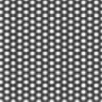
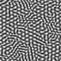
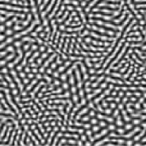
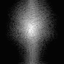
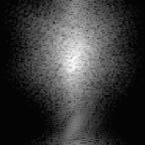
FIG. 6.: Numerical simulations of Eqs. (4) in a box of length $L=35$ ($K_{min}=0.1795$) with $128\times 128$ Fourier modes, for the values of the parameters $\nu=2$, $\tilde{\nu}=0.1$, $\alpha_{1}=\alpha_{2}=0$, $\tilde{\alpha}=1.5$, $\mu=3$ and $K=-4K_{min}$ (cf. Fig. 5d). The top panels show a reconstruction of the hexagonal pattern $\Psi=\sum^{3}_{i=1}A_{i}e^{i{\bf k}^{c}_{i}\cdot{\bf x}}$ with $k_{c}=20K_{min}$ for the times $t=32$, $t=52$ and $t=56$. In the bottom panels the corresponding Fourier spectra of the amplitude $A_{1}$ are shown. Note the shifting of the peak of the distribution to ever larger $y$-components of the wavevector.

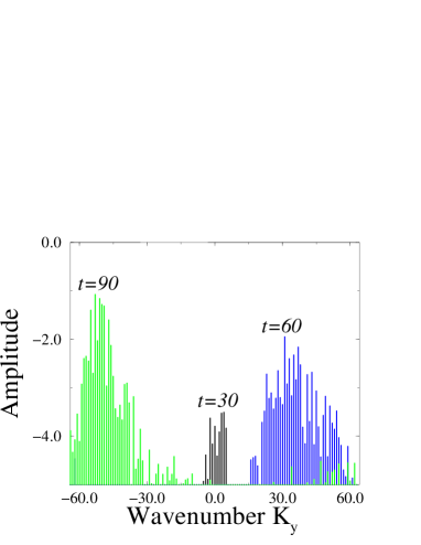
FIG. 7.: A cut of the Fourier spectrum (in logarithmic scale) of the amplitude $A_{1}$ at $K_{x}=0$ for the same parameters as in Fig. 6. As time progresses the peak of the distribution evolves towards higher wavenumbers and eventually reemerges at the negative end of the spectrum.

VI Conclusion

In this article we have analyzed the effect of chiral symmetry-breaking on the stability of hexagonal patterns. Such patterns arise, for instance, in non-Boussinesq Rayleigh-Bénard convection and in Marangoni convection, where the chiral symmetry can be broken by rotating the system. Focussing on the regime near threshold we have used the appropriate Ginzburg-Landau equations for the three modes making up the hexagon pattern. The chiral symmetry breaking introduces an asymmetry between the cubic coupling coefficients as well as a new nonlinear gradient term. The general linear stability analysis of these equations revealed long-wave as well as short-wave instabilities. The long-wave instabilities, which are captured with coupled phase equations, can be steady or oscillatory. For all parameter regimes investigated, the short-wave instabilities arise for larger values of the control parameter, but below the transition to oscillating hexagons. They can be due to the translation or the Hopf modes. In the latter case they are always oscillatory.

In contrast to the Küppers-Lortz instability of stripe patterns [1], no regime was identified in which hexagon patterns become unstable at all wavelengths. Nevertheless, persistent irregular dynamics of disordered hexagon patterns can apparently arise from the short-wave instability. Our numerical simulations of the Ginzburg-Landau equations indicate that the nonlinear evolution ensuing from the instability tends to introduce modes with wavevectors covering the whole critical circle. Of course, such a state in which the Fourier modes are distributed almost isotropically over the critical circle cannot be described by Ginzburg-Landau equations, since they break the isotropy at the very outset. This suggests the use of Swift-Hohenberg-type equations, which preserve the isotropy of the system. They are often used as truncated model equations (e.g. [35]) to study the qualitative behavior of systems, but can under certain conditions also be derived from the basic (fluid) equations as a long-wave description [36, 37, 38]. Recently, in such investigations of hexagons with broken chiral symmetry spatio-temporally chaotic states have been found to arise from the corresponding oscillatory short-wave instability [34]. As in our simulations of the Ginzburg-Landau equations the spatio-temporal chaos persists although for the same parameters there exist also stable ordered hexagon patterns. This bistability is somewhat reminiscence of the coexistence of spiral-defect chaos and ordered roll convection in Rayleigh-Bénard convection without rotation [39]. In the Swift-Hohenberg model the oscillatory short-wave instability can also lead to a supercritical bifurcation to hexagons that are modulated periodically in space and time [34]. No such state could be identified in the Ginzburg-Landau equations discussed here.

Our results suggest that rotation may induce irregular dynamics in hexagonal convection patterns quite close to threshold. So far, disordered hexagon patterns (without broken chiral symmetry) have been found in Marangoni convection [40] far from threshold and also in experiments on chemical Turing patterns [41]. In the latter case they appear to be due to the competition with the stripe pattern in a bistable regime.

From previous work it is well known that the chiral symmetry breaking delays the transition from hexagons to stripe patterns. More specifically, the steady bifurcation to the unstable mixed state is replaced by a Hopf bifurcation to a state of coherently oscillating hexagons [18, 19, 20]. Their side-band instabilities can be investigated with the same Ginzburg-Landau equations as discussed here [42].

- [1] G. Küppers and D. Lortz, J. Fluid Mech. 35, 609 (1969).
- [2] G. Küppers, Phys. Lett. A 32, 7 (1970).
- [3] F. Busse and K. Heikes, Science 208, 173 (1980).
- [4] F. Zhong, R. Ecke, and V. Steinberg, Physica D 51, 596 (1991).
- [5] F. Zhong and R. Ecke, Chaos 2, 163 (1992).
- [6] L. Ning and R. Ecke, Phys. Rev. E 47, 3326 (1993).
- [7] Y. Hu, R. Ecke, and G. Ahlers, Phys. Rev. Lett. 74, 5040 (1995).
- [8] Y. Hu, W. Pesch, G. Ahlers, and R. Ecke, Phys. Rev. E 58, 5821 (1998).
- [9] H. Xi, J. Gunton, and G. Markish, Physica A 204, 741 (1994).
- [10] Y. Tu and M. Cross, Phys. Rev. Lett. 69, 2515 (1992).
- [11] M. Fantz, R. Friedrich, M. Bestehorn, and H. Haken, Physica D 61, 147 (1992).
- [12] M. Neufeld, R. Friedrich, and H. Haken, Z. Phys. B 92, 243 (1993).
- [13] T. Clune and E. Knobloch, Phys. Rev. E 47, 2536 (1993).
- [14] M. Cross, D. Meiron, and Y. Tu, Chaos 4, 607 (1994).
- [15] Y. Ponty, T. Passot, and P. Sulem, Phys. Fluids 9, 67 (1997).
- [16] J. Millán-Rodríguez et al., Phys. Rev. Lett. 74, 530 (1995).
- [17] K. Bajaj, J. Liu, B. Naberhuis, and G. Ahlers, Phys. Rev. Lett. 81, 806 (1998).
- [18] J. Swift, in Contemporary Mathematics Vol. 28 (American Mathematical Society, Providence, 1984), p. 435.
- [19] A. Soward, Physica D 14, 227 (1985).
- [20] J. Millán-Rodríguez et al., Phys. Rev. A 46, 4729 (1992).
- [21] D. Riahi, Int. J. Eng. Sci. 32, 877 (1994).
- [22] M. Sushchik and L. Tsimring, Physica D 74, 90 (1994).
- [23] M. Golubitsky, J. Swift, and E. Knobloch, Physica D 10, 249 (1984).
- [24] S. Chandrasekhar, Hydrodynamic and Hydromagnetic Stability (Clarendon, Oxford, 1961).
- [25] Y. Pomeau, Physica D 23, 3 (1986).
- [26] H. Brand, Prog. Theor. Phys. Suppl. 99, 442 (1989).
- [27] G. Gunaratne, Q. Ouyang, and H. Swinney, Phys. Rev. E 50, 2802 (1994).
- [28] B. Echebarria and C. Pérez-García, Europhys. Lett. (1998).
- [29] J. Lauzeral, S. Metens, and D. Walgraef, Europhys. Lett. 24, 707 (1993).
- [30] R. Hoyle, Appl. Math. Lett. 9, 81 (1995).
- [31] P. Manneville, Dissipative Structures and Weak Turbulence (Academic Press, Boston, 1990).
- [32] J. Swift and P. Hohenberg, Phys. Rev. A 15, 319 (1977).
- [33] R. Graham, Phys. Rev. Lett. 76, 2185 (1996).
- [34] F. Sain and H. Riecke, in preparation .
- [35] M. Bestehorn and R. Friedrich, Phys. Rev. E 59, 2642 (1999).
- [36] E. Knobloch, Physica D 41, 450 (1990).
- [37] S. Cox, SIAM J. Appl. Math. 58, 1338 (1998).
- [38] A. Mancho, F. Sain, and H. Riecke, unpublished .
- [39] S. Morris, E. Bodenschatz, D. Cannell, and G. Ahlers, Phys. Rev. Lett. 71, 2026 (1993).
- [40] A. Thess and S. Orszag, J. Fluid Mech. 283, 201 (1995).
- [41] Q. Ouyang and H. Swinney, Chaos 1, 411 (1991).
- [42] B. Echebarria and H. Riecke, unpublished .