Quadratic Solitary Waves in a Counterpropagating Quasi-Phase-Matched Configuration

Abstract

We demonstrate the possibility of self-trapping of optical beams by use of quasi phase matching in a counterpropagating configuration in quadratic media. We also show the predominant stability of these spatial self-guided beams and estimate the power level required for their experimental observation.

Self-guided optical beams (or spatial solitons) have attracted significant research interest because they offer the possibility of all-optical switching and controlling light by light (see, e.g., [1]). During the past few years it has been realised that quadratic nonlinearity is particularly attractive for potential practical realizations of all-optical switching, in that it not only supports stable solitons both in planar waveguides and bulk media but also provids an ultra-fast electronic nonlinear response (see, e.g., [2]). The advantages of quadratic nonlinear materials are hampered in part by difficulties in obtaining close phase-velocity matching between interacting waves. One of the most effective ways to achieve such matching is the use of the so-called quasi-phase-matching (QPM) technique, in which large wave-vector mismatch between interacting waves is compensated for by periodic alternation of the sign of effective $\chi^{(2)}$ coefficient. This technique has been known since 1962, Ref. [3], but only in the past decade has technological progress put the QPM technique in the front line of modern nonlinear optics [4]. In spite of all the theoretical and experimental progress achieved in the field of quadratic solitons, only solitons formed by waves with the same direction of propagation have been analysed so far (conventional co-propagating configuration; see, e.g., [2, 5]). In a few works the advantages and implications of QPM technique for this type of solitons have been analysed specifically [6]. However, a parametric interaction between counterpropagating quasi-phase-matched waves in quadratic [$\chi^{(2)}$] media is also possible. Corresponding analysis made for for non-soliton (plane wave interaction) case [7] revealed certain advantages of a counterpropagating interaction system over conventional copropagating strategies. Moreover, recently a very similar so-called backward QPM configuration has been investigated experimentally (see [8]). In this work we investigate the QPM counterpropagating scheme, searching for solitary waves and investigating their stability.

We consider the interaction between four optical waves in a slab waveguide with an appropriate nonlinear grating. Two forward-propagating waves, the fundamental at frequency $\omega$ and with wave number $k_{\omega}$ and the second harmonic ($2\omega,k_{2\omega}$), are coupled with two backward-propagating ones, the fundamental ($\omega,-k_{\omega}$) and the second harmonic ($2\omega,-k_{2\omega}$) [see Fig. 1, (a)]. Spatial modulation of nonlinear susceptibility along a crystal can be described in terms of square-wave function $d(z)$ [see Fig. 1, (b)]. In this case the only nonzero matrix elements of the Fourier transform of $d(z)$ are given by: $d_{l}=-2i/(\pi l)$, where $l=2m-1$, $m=\pm 1,\pm 2,\pm 3\dots$ Following the method developed in Ref. [6] we can derive the corresponding normalised system of equations which has the following dimensionless form:

$$\begin{array}[]{r}i\frac{\textstyle\partial E_{\omega}^{+}}{\textstyle\partial z}+\frac{\textstyle\partial^{2}E_{\omega}^{+}}{\textstyle\partial x^{2}}-\alpha_{+}E_{\omega}^{+}+A_{2\omega}E_{\omega}^{-*}=0,\vspace{1 mm}\\ -i\frac{\textstyle\partial E_{\omega}^{-}}{\textstyle\partial z}+\frac{\textstyle\partial^{2}E_{\omega}^{-}}{\textstyle\partial x^{2}}-\alpha_{-}E_{\omega}^{-}+A_{2\omega}E_{\omega}^{+*}=0,\vspace{1 mm}\\ i\sigma\frac{\textstyle\partial E_{2\omega}^{+}}{\textstyle\partial z}+\frac{\textstyle\partial^{2}E_{2\omega}^{+}}{\textstyle\partial x^{2}}-\sigma\beta_{+}E_{2\omega}^{+}+A_{\omega}^{+}E_{\omega}^{-}=0,\vspace{1 mm}\\ -i\sigma\frac{\textstyle\partial E_{2\omega}^{-}}{\textstyle\partial z}+\frac{\textstyle\partial^{2}E_{2\omega}^{-}}{\textstyle\partial x^{2}}-\sigma\beta_{-}E_{2\omega}^{-}+A_{\omega}^{-}E_{\omega}^{+}=0,\end{array}\vspace*{- 2mm}$$ (1)

where $A_{2\omega}\equiv(d_{-l}E_{2\omega}^{+}+d_{l}E_{2\omega}^{-})$, $A_{\omega}^{+}\equiv 2d_{l}E_{\omega}^{+}$, $A_{\omega}^{-}\equiv 2d_{-l}E_{\omega}^{-}$, $\beta_{+}\equiv\alpha_{+}-\alpha_{-}+\delta$, $\beta_{-}\equiv\alpha_{-}-\alpha_{+}+\delta$; $E^{\pm}_{\omega}(x,z),E^{\pm}_{2\omega}(x,z)$ are the envelopes of the fundamental wave and its second harmonic, respectively, sign ”+” (”–”) corresponds to the forward (backward) propagating wave; $x$ is the transverse coordinate normalised on the width of the beam $r_{0}$; $z$ is the propagation distance which is normalised on the diffraction length $z_{d}=k_{2\omega}r_{0}^{2}$; parameters $\alpha_{+}$ and $\alpha_{-}$ are nonlinear induced propagation constant shifts of the fundamental waves. Other two system parameters, $\sigma\equiv k_{2\omega}/k_{\omega}=2$ and $\delta\equiv(2\pi l/L-k_{2\omega})z_{d}$ (where $L$ is the period of the nonlinear grating and $l$ is the order of QPM), are defined by the particular experimental setup. Note, that in contrast to Ref. [6] we have omitted all effective cubic terms in Eqs. (1). This is well justified for lower order QPM (for $l<15$) because in this case the cubic terms would become noticeable only when the light intensity exceeds the damage threshold for the typical nonlinear crystal.

The system (1) has the following family of power-like integrals of motion:

$$\begin{array}[]{c}Q(p_{1},p_{2})=\int_{-\infty}^{+\infty}\{2p_{1}|E_{\omega}^{+}|^{2}+2p_{2}|E_{\omega}^{-}|^{2}+\\ +\sigma(p_{1}-p_{2})(|E_{2\omega}^{+}|^{2}-|E_{2\omega}^{-}|^{2})\}\,dx,\end{array}$$ (2)

where $p_{1},\>p_{2}$ are any real numbers. Using the asymptotic expansion technique and the method based on integrals of motion (see Ref. [9]) one can demonstrate that the stability threshold for the fundamental family of stationary localised solutions of the system (1) is given as:

$$\frac{\partial(Q_{1},Q_{2})}{\partial(\alpha_{+},\alpha_{-})}=\frac{\partial Q_{1}}{\partial\alpha_{+}}\frac{\partial Q_{2}}{\partial\alpha_{-}}-\frac{\partial Q_{1}}{\partial\alpha_{-}}\frac{\partial Q_{2}}{\partial\alpha_{+}}=0,$$ (3)

where $Q_{1}$, $Q_{2}$ are any two linearly independent invariants from the family (2), calculated for the fundamental stationary solitons, e.g. $Q_{1}=Q(1,0)$ and $Q_{2}=Q(0,1)$. More elaborate analysis shows that for the instability domains either of the two following conditions is satisfied in the vicinity of stability-instability boundaries:

$$\frac{\partial Q_{1}}{\partial\alpha_{+}}(\frac{\partial Q_{1}}{\partial\alpha_{+}}\frac{\partial Q_{2}}{\partial\alpha_{-}}-\frac{\partial Q_{1}}{\partial\alpha_{-}}\frac{\partial Q_{2}}{\partial\alpha_{+}})<0,$$ (4)

$$\frac{\partial Q_{2}}{\partial\alpha_{-}}(\frac{\partial Q_{1}}{\partial\alpha_{+}}\frac{\partial Q_{2}}{\partial\alpha_{-}}-\frac{\partial Q_{1}}{\partial\alpha_{-}}\frac{\partial Q_{2}}{\partial\alpha_{+}})<0.\$$ (5)

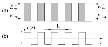
FIG. 1.: Parametric interaction of counterpropagating waves. (a) Nonlinear grating is used to couple forward- (”+”) and backward-propagating (”–”) waves; (b) square-wave function $d(z)$ approximates the periodic modulation of the effective second order nonlinear susceptibility coefficient.

At $\alpha_{+}=\alpha_{-}$ and $\delta=\sigma\alpha_{+}/2$ the system (1) has an exact analytical stationary localised solution in the form of $E^{\pm}_{\omega,s}(x)=3\alpha_{+}/[4|d_{l}|{\rm cosh}^{2}(\sqrt{\alpha_{+}}x/2)]$, $E^{\pm}_{2\omega,s}(x)=\mp iE^{\pm}_{\omega,s}(x)$. For other values of the parameters, analytical expressions cannot be found and numerics should be used. For numerical analysis it is more convenient to renormalise the system (1) reducing the number of parameters. As a result we obtain the system

$$\begin{array}[]{r}i\frac{\textstyle\partial V^{+}}{\textstyle\partial Z}+\frac{\textstyle\partial^{2}V^{+}}{\textstyle\partial X^{2}}-V^{+}+(W^{+}+W^{-})V^{-*}=0,\vspace{1 mm}\\ -i\frac{\textstyle\partial V^{-}}{\textstyle\partial Z}+\frac{\textstyle\partial^{2}V^{-}}{\textstyle\partial X^{2}}-\gamma V^{-}+(W^{+}+W^{-})V^{+*}=0,\vspace{1 mm}\\ i\sigma\frac{\textstyle\partial W^{+}}{\textstyle\partial Z}+\frac{\textstyle\partial^{2}W^{+}}{\textstyle\partial X^{2}}-\sigma\beta_{W}^{+}W^{+}+2V^{+}V^{-}=0,\vspace{1 mm}\\ -i\sigma\frac{\textstyle\partial W^{-}}{\textstyle\partial Z}+\frac{\textstyle\partial^{2}W^{-}}{\textstyle\partial X^{2}}-\sigma\beta_{W}^{-}W^{-}+2V^{+}V^{-}=0,\end{array}$$ (6)

where $\beta_{W}^{+}\equiv 1-\gamma+\alpha$, $\beta_{W}^{-}\equiv\gamma-1+\alpha$. The connection between Eqs. (1) and Eqs. (6) is given by scaling $E_{\omega}^{\pm}=\alpha_{+}V^{\pm}/|d_{l}|$, $\>E_{2\omega}^{\pm}=\mp i\alpha_{+}W^{\pm}/|d_{l}|$, $\>x=X/\sqrt{\alpha_{+}}$, $\>z=Z/\alpha_{+}$. System (6) has only two parameters, defined as $\gamma\equiv\alpha_{-}/\alpha_{+}$, $\>\alpha\equiv\delta/\alpha_{+}$. Stationary solitons of the system (6) can be found numerically, e.g., using the relaxation technique, for all $\gamma>0$, $\beta_{W}^{\pm}>0$. Some examples of stationary solitons of the system (6) are shown in Fig. 2.

Criteria (3), (4) can be rederived for the system (6), and then used to calculate the boundary of stability area in the $(\alpha,\gamma)$ plane. For the precise calculations of the invariants we use the tangential transformation of transverse soliton coordinate $X=\tan\pi\tilde{X}$, Ref.[10]. Using this map we cover the infinite interval in $X$ $(-\infty~{}<~{}X~{}<~{}\infty)$ by a finite one in $\tilde{X}$ $(-1/2~{}<~{}\tilde{X}~{}<~{}1/2)$.

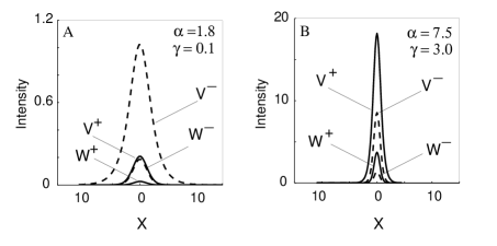
FIG. 2.: Examples of stationary solitons due to counterpropagating QPM configuration. Profiles are calculated for the system (6). Solid curves correspond to the forward set of waves, dashed lines - to the backward-propagating ones.

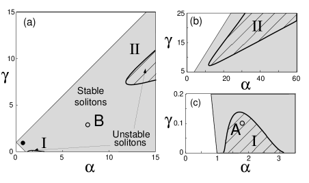
FIG. 3.: (a) Existence and stability diagram for the stationary solutions of the system (6). Solid curves are defined by the stability threshold condition (3); (b), (c) enlarged plots of the unstable regions I and II. Soliton profiles calculated for the points A and B are shown in Fig. 2. Filled circle corresponds to the exact solution (see text).

To confirm the validity of the stability results given by Eqs. (3) and (4) we analyse numerically an eigenvalue-eigenvector problem corresponding to Eqs. (6) linearised about stationary solitons of interest. In all analysed cases the theoretically predicted stability-instability properties were confirmed numerically. However, we should note that the theoretical approach which we use does not describe so-called oscillatory instabilities (see, e.g., [11]) and, although we have not detected such instabilities numerically, further analysis is necessary to completely rule out their possibility. The stability/instability domains given by criteria (3) and (4) are shown in Fig. 3. Direct numerical modelling of Eqs. (6) confirms the results of our stability analysis. Two examples of propagation of unstable solitons are presented in Fig. 4.

Optical power required for generation of counterpropagating solitons of a given beam width can be estimated by the method proposed in Ref. [13]. After defining the soliton width $R_{s}$ as the maximum width at the half-maximum of the the second harmonic amplitude $E_{2\omega}^{+}$ the conditional minimum $\tilde{Q}_{min}$ of the total power functional $\tilde{Q}(\alpha,\gamma)=R_{s}^{3/2}\int_{-\infty}^{+\infty}\!\{|V^{+}|^{2}+|V^{-}|+2\sigma|W^{+}|^{2}+2\sigma|W^{-}|^{2}\}\,dX$ has to be found. Then minimal power density $I_{min}$ can be calculated as:

$$I_{min}=\tilde{Q}_{min}\frac{L_{eff}}{4\pi\chi^{2}_{bulk}r_{0}^{4}|d_{l}|^{2}},$$ (7)

where nonlinear coefficient $\chi_{bulk}=(\omega^{2}/c^{2})(2/c\epsilon_{0}n)^{1/2}\chi^{(2)}$ is expressed in $W^{-1/2}cm^{-1}$, $\chi^{(2)}$ is the effective element of the second order susceptibility tensor, $L_{eff}$ is the width of a waveguide. For the first order QPM, i.e. $l=1$, and the values from Ref. [5]: $r_{0}=20\mu m$, $\lambda=2\pi c/\omega\simeq 1.064\mu m$, refractive index $n\simeq 1.79$, $\chi^{(2)}\approx 6pm/V$ and a waveguide with effective width $L_{eff}$ about $1\mu m$, we obtain $I_{min}\approx 2.8\;W/\mu m$ ($\tilde{Q}_{min}\approx 103$ at $\alpha=3.15,\gamma=1.00$).

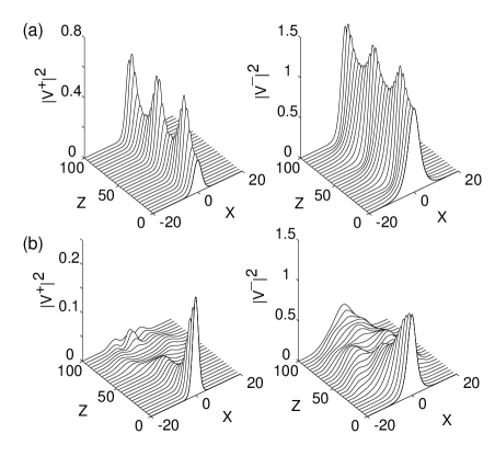
FIG. 4.: Examples of unstable propagation of a slightly perturbed stationary soliton shown in Fig. 2, A. Two typical kinds of instability correspond to slightly increased, (a), and reduced, (b), soliton amplitudes. Unstable soliton with a slightly increased amplitude is clearly evolving to some stable state with an excited internal mode (see, e.g., [12]).

Our analysis shows that the point of optimal generation is in the domain of stability and corresponds to $V^{+}=V^{-}$ and $W^{+}=W^{-}$, i.e., one can generate the whole four-wave soliton using only two seeded forward-propagating waves at one end of a crystal and a mirror on the other [the use of mirror will also halve the generation threshold (7)]. Thus the solitons due to counterpropagating QPM, in principle, require less optical power for an experimental observation in comparison with conventional quadratic solitons, for which the corresponding value is $I_{min}\approx 3.4\;W/\mu m$ (see Ref. [13]). In practice lowering the generation threshold requires a very short (sub-micron) grating period to arrange for lower order QPM. This was not the case for the experiments [8] where the grating period was about $3\mu m$ and QPM order was high. However, experimental progress in quantum well technology (see, e.g., [14]) may make lower order counterpropagating QPM experimentally possible in the near future.

In conclusion, we have demonstrated the existence of solitons that are due to counterpropagating QPM in quadratic media. We obtained an analytic criterion for the stability threshold for these solitons and found a substantial region of stability with only two small regions of unstable solitons. We also discussed the conditions for experimental observation of these novel solitons.

The authors thank V. V. Steblina for helpful discussions and suggestions. A.V.B. and R.A.S. acknowledge support from the Australian Research Council.

REFERENCES

- [1] M. Segev and G. I. Stegeman, Physics Today 51, No. 8, 42 (1998), and references therein.
- [2] G. I. Stegeman, D. J. Hagan, and L. Torner, J. Opt. Quantum Electron. 28, 1691 (1996).
- [3] J. A. Armstrong, N. Bloembergen, J. Ducuing, P. S. Pershan, Phys. Rev. 127, 1918 (1962).
- [4] M. M. Fejer, G. A. Magel, D. H. Jundt, R. L. Byer, IEEE J. Quant. Electron. 28, 2631 (1992); G. M. Miller, R. G. Batchko, W. M. Tulloch, D. R. Weise, M. M. Fejer, R.L. Byer, Opt. Lett. 22, 1834 (1997).
- [5] W. E. Torruellas, Z. Wang, D. J. Hagan, E. W. Van Stryland, G. I. Stegeman, L. Torner, C. R. Menyuk, Phys. Rev. Lett. 74, 5036 (1995); V. V. Steblina, Yu. S. Kivshar, A. V. Buryak, Opt. Lett. 23, 156 (1998); B. Costantini, C. De Angelis, A. Barthelemy, B. Bourliaguet, V. Kermene, Opt. Lett. 23, 424 (1998).
- [6] C. B. Clausen, O. Bang, Yu. Kivshar, Phys. Rev. Lett. 78, 4749 (1997); M. Cha, Opt. Lett. 23, 250 (1998); C. B. Clausen, L. Torner, Opt. Lett., 24, 7 (1999).
- [7] Y. J. Ding, J. B. Khurgin, Opt. Lett. 21, 1445 (1996); G. D. Landry, T. A. Maldonado, Appl. Opt. 37, 7809 (1998).
- [8] J. B. Kang, Y. J. Ding, W. K. Burns, J. S. Melinger, Opt. Lett., 22, 862 (1997); X. Gu, R. Y. Korotkov, Y. J. Ding, J. U. Kang, J. B. Khurgin, J. Opt. Soc. Am. B, 15, 1561 (1998).
- [9] A. V. Buryak, Y. Kivshar, S. Trillo, Phys. Rev. Lett. 77, 5210 (1996).
- [10] S. J. Hewlett, F. Ladouceur, J. Lightwave Tech. 13, 375 (1995).
- [11] I. V. Barashenkov, D. E. Pelenovsky, and E. V. Zemlyanaya, Phys. Rev. Lett. 80, 5117 (1998); A. De Rossi, C. Conti, and S. Trillo, Phys. Rev. Lett. 81, 85 (1998).
- [12] Yu. S. Kivshar, D. E. Pelenovsky, T. Cretegny, and M. Peyrard, Phys. Rev. Lett. 80, 5032 (1998).
- [13] A. V. Buryak, Yu. S. Kivshar, S. Trillo, J. Opt. Soc. Am. B 14, 3110 (1997).
- [14] O. A. Aktsipertov, P. V. Elyutin, E. V. Malinnikova, E. D. Mishina, A. N. Rubtsov, W. de Jong, and Th. Raising, Physics-Doklady, 42, 340 (1997); R. C. Tu, Y. K. Su, and S. T. Chou, J. of Appl. Phys., 85, 2398 (1999).