Existence threshold for the ac-driven damped nonlinear Schrödinger solitons

Abstract

It has been known for some time that solitons of the externally driven, damped nonlinear Schrödinger equation can only exist if the driver’s strength, $h$, exceeds approximately $(2/\pi)\gamma$, where $\gamma$ is the dissipation coefficient. Although this perturbative result was expected to be correct only to the leading order in $\gamma$, recent studies have demonstrated that the formula $h_{\rm thr}=(2/\pi)\gamma$ gives a remarkably accurate description of the soliton’s existence threshold prompting suggestions that it is, in fact, exact. In this note we evaluate the next order in the expansion of $h_{\rm thr}(\gamma)$ showing that the actual reason for this phenomenon is simply that the next-order coefficient is anomalously small: $h_{\rm thr}=(2/\pi)\gamma+0.002\gamma^{3}$. Our approach is based on a singular perturbation expansion of the soliton near the turning point; it allows to evaluate $h_{\rm thr}(\gamma)$ to all orders in $\gamma$ and can be easily reformulated for other perturbed soliton equations.

I Introduction

The externally driven, damped nonlinear Schrödinger (NLS) equation,

$$i\Psi_{t}+\Psi_{xx}+2|\Psi|^{2}\Psi=-i\gamma\Psi-he^{i\Omega t},$$ (1)

arises in a variety of fields including plasma and condensed matter physics, nonlinear optics and superconducting electronics. In some of these applications (e.g. in the study of the optical soliton propagation in a diffractive or dispersive ring cavity in the presence of an input forcing beam [3]; in the description of easy-axis ferromagnets in an external rotating magnetic field perpendicular to the easy axis [4]; in the theory of rf-driven waves in plasma [5]) Eq.(1) has a direct interpretation. In others — like for instance in charge-density-wave conductors with external electric field [6]; shear flows in nematic liquid crystals [7]; ac-driven long Josephson junctions [8], and periodically forced Frenkel-Kontorova chains [9] — it occurs as an amplitude equation for small and slowly changing solutions of the externally driven, damped sine-Gordon equation:

$$q_{tt}+\lambda q_{t}-q_{xx}+\sin q=\Gamma\cos(\omega t).$$

Without loss of generality $\Omega$ in Eq.(1) can be normalized to unity [10, 11, 12]; hence, the driver’s strength $h$ and dissipation coefficient $\gamma$ are the only two essential control parameters. Given some $h$ and $\gamma$, a fundamental question is what nonlinear attractors will arise at this point of the $(\gamma,h)$-plane. In their pioneering paper [13] Kaup and Newell considered Eq.(1) on the infinite line under the vanishing boundary conditions at infinity. By means of the Inverse Scattering-based perturbation theory, these authors have demonstrated that for small $h$ and $\gamma$ Eq.(1) exhibits two soliton solutions phase-locked to the frequency of the driver. As $h$ is decreased for the fixed $\gamma$, the two solitons approach each other and eventually merge in a turning point for $h=(2/\pi)\gamma$ [13]. Consequently, this value plays the role of a threshold; no solitons exist below $h=(2/\pi)\gamma$. Later the same existence threshold was reobtained by Terrones, McLaughlin, Overman and Pearlstein [11] in a regular perturbation construction of solutions to (1) in powers of $h$ and $\gamma$ (see also [14]).

In ref.[12] equation (1) was studied, numerically, in the full range of $h$ and $\gamma$. It was found that the two soliton solutions persist for $\gamma$ up to approximately $0.7$. For each $\gamma\lesssim 0.7$ there is a turning point at some $h=h_{\rm thr}$ at which one branch of solitons turns into another, and which plays the role of the lower boundary of the existence region [15]. Amazingly, Kaup and Newell’s approximate relation $h_{\rm thr}=(2/\pi)\gamma$ was found to remain valid even for not very small $\gamma$. For example, for $\gamma=0.48$ the ratio $h_{\rm thr}/\gamma$ is different from $2/\pi$ by only one part in a thousand [12].

A completely different approach was put forward by Kollmann, Capel and Bountis [16] who regarded Eq.(1) as the continuous limit of a discrete NLS equation which they studied by means of the fixed point analysis and the Melnikov-function method. In particular, the lower boundary was obtained from the tangential intersection of the invariant manifolds of a hyperbolic fixed point. A remarkable accuracy of Kaup and Newell’s linear law detected in [12] as well as conclusions of their own Melnikov-function analysis prompted the authors of [16] to suggest that the relation $h_{\rm thr}=(2/\pi)\gamma$ can be exact, at least for sufficiently small $\gamma$.

The aim of the present note is to demonstrate that this relation is, in fact, not exact, and the actual reason why it appears to be so accurate for small $\gamma$ is simply because the coefficient of the next term in the expansion of $h_{\rm thr}(\gamma)$ in powers of $\gamma$ is anomalously small. We do this by reconstructing the two solitons in the vicinity of the lower boundary of their existence domain by means of a singular (rather than regular) perturbation expansion. This novel expansion constitutes the main technical achievement of our work; its scope of applicability is obviously much wider than just the damped-driven NLS equation (1).

The reason why the regular expansion is not adequate near the solitons’ existence boundary is quite simple. The point is that the regular expansion is based on the assumption that solutions can be continued along rays $h={\mathfrak{h}}\gamma$ (${\mathfrak{h}}=\mbox{const}$.) But since the boundary is not exactly a straight line $h=(2/\pi)\gamma$ (as will be shown below, it slowly recedes upwards from this straight line), the ray $h={\mathfrak{h}}\gamma$ with ${\mathfrak{h}}$ slightly above $2/\pi$ will hit the boundary at some small $\gamma=\gamma_{0}$. Consequently, the regular expansion fails to continue the solution beyond $\gamma_{0}$. In the singular expansion, on the other hand, the solution is continued along a curve whose shape is calculated simultaneously with finding perturbative corrections to the solution itself. In this way the existence boundary can be found to any desirable accuracy. (In this paper we restrict ourselves to terms $\sim\gamma^{3}$.) This idea should remain applicable to other perturbed soliton-bearing equations.

The outline of this paper is as follows. We start by discussing the regular asymptotic expansion as $h$ and $\gamma\to 0$ (section II). The procedure is similar to the one in [11]; the only difference is that since we now deal with solutions decaying at infinities ($\Psi_{x}\to 0$) rather than periodic as in [11], we will be able to find perturbative corrections in closed form. In section III we explain why the perturbation series for $\Psi$ breaks down as $h$ approaches the turning point, and replace it by a singular expansion. This allows us to find the next terms in the expansion of $h_{\rm thr}(\gamma)$. The resulting asymptotic formula is compared then with the threshold $h_{\rm thr}(\gamma)$ obtained in a high-precision numerical analysis of Eq.(3) for several values of $\gamma$. Next, after we have achieved an understanding of why the regular expansion fails and how it can be cured near the existence threshold, a natural step is to try to develop a unified expansion which would be equally applicable near and far from the threshold. This is done in section IV. Finally, some concluding remarks are made in section V followed by a brief summary of our results.

II Regular perturbation expansion

By making a substitution $\Psi(x,t)=\psi(x,t)e^{it}$ Eq.(1) can be reduced to an autonomous equation

$$i\psi_{t}+\psi_{xx}+2|\psi|^{2}\psi-\psi=-i\gamma\psi-h.$$ (2)

We will be interested in time-independent solutions of Eq.(2); these satisfy the stationary equation

$$\psi_{xx}+2|\psi|^{2}\psi-\psi=-i\gamma\psi-h$$ (3)

with the boundary conditions

$$\psi_{x}(x)\rightarrow 0\quad{\rm as}\ |x|\rightarrow\infty.$$

We start with developing a regular perturbation expansion away from the turning point. As the authors of [11], we assume that we are approaching the origin on the ($\gamma,h$)-plane along a straight line $h={\mathfrak{h}}\gamma$ where ${\mathfrak{h}}$ is a proportionality coefficient. Letting

$$\psi=(u+iv)e^{-i\alpha},$$ (5)

where $\alpha$ is some constant phase that can be conveniently chosen at a later stage, we expand

$$u=u_{0}+\gamma u_{1}+...,\quad v=v_{0}+\gamma v_{1}+...$$ (6)

and substitute into Eq.(3). The coefficient of $\gamma^{0}$ gives the unperturbed stationary NLS equation with a well-known soliton solution

$$\left(\begin{array}[]{c}u_{0}\\ v_{0}\end{array}\right)=\left(\begin{array}[]{c}\cos\theta\\ \sin\theta\end{array}\right){\rm sech}x.$$ (11)

Here $\theta$ is a free parameter. Next, at the order $O(\gamma^{1})$ one gets

$${\hat{H}}_{0}\left(\begin{array}[]{c}u_{1}\\ v_{1}\end{array}\right)=\left(\begin{array}[]{c}{{\mathfrak{h}}}\cos\alpha-v_{0}\\ {{\mathfrak{h}}}\sin\alpha+u_{0}\end{array}\right),$$ (16)

where the Hermitean operator

$${\hat{H}}_{0}\equiv\left(-\frac{\partial^{2}}{\partial x^{2}}+1\right){\hat{I}}-2\left(\begin{array}[]{lr}v_{0}^{2}+3u_{0}^{2}&2u_{0}v_{0}\\ 2u_{0}v_{0}&u_{0}^{2}+3v_{0}^{2}\end{array}\right)$$ (19)

and ${\hat{I}}$ is the $2\times 2$ identity matrix. In order for the equation (16) to be solvable in the class of bounded functions, its right-hand side needs to be orthogonal to the vector $(v_{0},-u_{0})^{T}$, the eigenfunction of the operator ${\hat{H}}_{0}$ associated with the zero eigenvalue. (This zero eigenvalue results from the U(1) phase-invariance of the unperturbed NLS equation.) The orthogonality gives a relation between $\alpha$ and $\theta$,

$$\pi{{\mathfrak{h}}}\sin(\theta-\alpha)=2,$$ (20)

implying that only one of the two parameters (say, $\theta$) can be chosen freely. It does not matter what exactly we choose for $\theta$; the net phase of the leading-order approximation is $(\theta-\alpha)$ and this is fixed by Eq.(20). The meaning of this relation is straightforward. For $h=\gamma=0$, the NLS equation has a family of soliton solutions, $\psi=e^{i(\theta-\alpha)}{\rm sech\/}x$, with $(\theta-\alpha)$ arbitrary. However, if we want to continue the solution along the line $h={\mathfrak{h}}\gamma$, the unperturbed solution that we need to start with has the phase given by Eq.(20).

It is convenient to take $\theta=\pi/2$; this makes the linear operator (19) diagonal. (The other diagonal choice $\theta=0$ is also acceptable but somewhat less convenient in the present context.) The constant phase $\alpha$ is then determined by

$$\cos\alpha=\frac{2}{\pi}\frac{1}{{\mathfrak{h}}}.$$ (21)

In fact, there are two values of $\alpha$ defined by this equation, one positive and one negative. The positive $\alpha=\alpha_{+}$ corresponds to the soliton $\psi^{(+)}$ and the negative $\alpha=\alpha_{-}$ defines the soliton $\psi^{(-)}$. Since the left-hand side cannot exceed 1, the right-hand side gives the well-known formula for the lower boundary of the domain of existence of the two solitons: ${{\mathfrak{h}}}\geq{{\mathfrak{h}}}_{\rm thr}=2/\pi$ [13, 11, 14]. (In the next section we will obtain a more precise formula for this threshold.)

Now for $\theta=\pi/2$ the equations (16) become

$$L_{0}u_{1}(x)={{\mathfrak{h}}}\cos\alpha-v_{0}(x);$$ (22)

$$L_{1}v_{1}(x)={{\mathfrak{h}}}\sin\alpha,$$ (23)

where $v_{0}(x)={\rm sech\/}x$ and $L_{0}$ and $L_{1}$ are the standard Schrödinger operators with familiar spectral properties:

$$L_{0}=-\partial^{2}/\partial x^{2}+1-2{\rm sech\/}^{2}x;$$ (24)

$$L_{1}=-\partial^{2}/\partial x^{2}+1-6{\rm sech\/}^{2}x.$$ (25)

The operator $L_{1}$ is invertible on even functions; in particular,

$$L_{1}^{-1}{\rm sech}\,x=\frac{1}{2}(x\,{\rm tanh}\,x-1){\rm sech\/}x,$$ (26)

$$L_{1}^{-1}{\rm sech}^{3}x=-\frac{1}{4}{\rm sech}x$$ (27)

and

$$L_{1}^{-1}1=1-2{\rm sech}^{2}x.$$ (28)

Hence Eq.(23) is readily solved:

$$v_{1}={{\mathfrak{h}}}\sin\alpha(1-2{\rm sech}^{2}x).$$ (29)

The condition (21) being in place, Eq.(22) is solved as well:

$$u_{1}={\cal U}_{1}(x)+A{\rm sech\/}x,$$ (31)

where

$${\cal U}_{1}(x)=\frac{2}{\pi}+\frac{1}{2}{\rm tanh}x\,{\rm sinh}x+\frac{1}{\pi}\times\{j(x)\,{\rm sech}x-$$ (32)

$$-(x\,{\rm sech}x+{\rm sinh}x)\,{\rm arcsin}({\rm tanh}x)-1\},$$ (33)

$$j(x)\equiv\int^{x}_{0}\xi\,{\rm sech}\xi\,d\xi,$$ (34)

and $A$ is an arbitrary constant which is to be fixed at higher orders of the expansion. Hence we proceed to $O(\gamma^{2})$ to find

$$L_{0}u_{2}=(4v_{0}u_{1}-1)v_{1},$$ (35)

$$L_{1}v_{2}=u_{1}+2v_{0}(u_{1}^{2}+3v_{1}^{2}).$$ (36)

Equation (35) is solvable if its right-hand side is orthogonal to ${\rm sech}x$. Substituting from (29)-(31), this condition fixes the constant $A$:

$$A=A^{(0)}\equiv\frac{4}{\pi}\int{\cal U}_{1}(x)\,{\rm sech}^{2}x(1-2{\rm sech}^{2}x)dx,$$ (37)

where we have used Eqs.(27-28). (Here we have written $A^{(0)}$ for $A$ so as to emphasize that this is now a fixed number; this number will reappear in the singular expansion below.) Eq.(35) is now solved in the form

$$u_{2}={\cal U}_{2}(x)+B{\rm sech}x.$$ (38)

The constant $B$ is to be fixed at the $\gamma^{3}$-level, where we obtain the equation

$$L_{0}u_{3}=2\{u_{1}(v_{1}^{2}+u_{1}^{2})+2v_{0}(u_{2}v_{1}+u_{1}v_{2})\}-v_{2}.$$ (39)

The solvability condition for eq.(39) gives us $B$:

$$B=(\pi{{\mathfrak{h}}}\sin\alpha)^{-1}\times$$ (40)

$$\int v_{0}\{2u_{1}(u_{1}^{2}+v_{1}^{2})+4v_{0}(u_{1}v_{2}+{\cal U}_{2}v_{1})-v_{2}\}\,dx.$$ (41)

So far our treatment followed the lines of Terrones et al [11]; the only difference is that our $v_{0},u_{1},v_{1},...$ are given by explicit formulas. Using (33) in (37) and integrating numerically, we identify the constant $A^{(0)}$ which completes the determination of the first-order corrections: $A^{(0)}=-2.4378\times 10^{-1}$.

Let us now send $h\to(2/\pi)\gamma$. The formula (29) for $u_{1}(x)$ is not affected and the expression (37) for $A$ remains valid as well. Therefore, the solvability of Eq.(35) is ensured and $u_{2}$ can be written in the form (38). The constant $B$ is expected to be identifiable from Eq.(41). However, for ${{\mathfrak{h}}}\to 2/\pi$ we have $\sin\alpha\to 0$ and so this formula gives $B=\infty$ unless

$$\int v_{0}(2u_{1}^{3}+4v_{0}u_{1}v_{2}-v_{2})dx=0.$$ (42)

(Here we have used that $v_{1}\to 0$ as $\sin\alpha\to 0$.) In general the condition (42) is not in place, and therefore the regular expansion blows up.

III Singular perturbation expansion at the turning point

The reason for the breaking down of the expansion is that it was implicitly assumed in Eq.(6) that $v_{1}=O(1)$ whereas in the actual fact, in the limit ${{\mathfrak{h}}}\to 2/\pi$ we have $v_{1}\to 0$. Let us now explicitly take this fact into account by writing

$$u=\gamma u_{1}+\gamma^{2}u_{2}...,\quad v=v_{0}+\gamma^{2}v_{2}+...,$$ (44)

where $v_{0}={\rm sech}x$. We also expand ${\mathfrak{h}}$:

$${{\mathfrak{h}}}={{\mathfrak{h}}}_{0}+{{\mathfrak{h}}}_{1}\gamma+{{\mathfrak{h}}}_{2}\gamma^{2}+....,\quad{{\mathfrak{h}}}_{0}=\frac{2}{\pi}.$$ (45)

(Thus we have fixed $\theta=\pi/2$ and $\alpha=0$ straight away.) Substituting into (3), the first order in $\gamma$ yields eq.(22) where one should only replace ${\mathfrak{h}}\cos\alpha\to{\mathfrak{h}}_{0}$. Its solution is given by the same eq.(29) as before, with $A$ an undetermined constant. At the order $\gamma^{2}$ we obtain

$\displaystyle L_{0}u_{2}={{\mathfrak{h}}}_{1},$

and hence ${{\mathfrak{h}}}_{1}=0$ and $u_{2}=B\,{\rm sech\/}x$. The equation for $v_{2}$ is now

$$L_{1}v_{2}=u_{1}+2v_{0}u_{1}^{2}$$ (46)

[cf. Eq.(36)]; this is always solvable. Finally, the $\gamma^{3}$-level yields

$\displaystyle L_{0}u_{3}=2(u_{1}^{3}+2v_{0}u_{1}v_{2})-v_{2}+{{\mathfrak{h}}}_{2}$

[cf. (39)], whose solvability condition is given by

$$\int v_{0}\,(2u_{1}^{3}+4v_{0}u_{1}v_{2}-v_{2}+{{\mathfrak{h}}}_{2})\,dx=0.$$ (47)

It turns out that it is only this equation (47) that fixes the constant $A$ in Eq.(31). Indeed, substituting $u_{1}$ from (31) and $v_{2}$ from (46), Eq.(47) reduces to a quadratic equation

$$A^{2}-2{P}A+{Q}-\pi{{\mathfrak{h}}}_{2}=0,$$ (48)

where after some algebra the coefficients are found to be

$${P}=-2{{\mathfrak{h}}}_{0}^{2}+\frac{{{\mathfrak{h}}}_{0}}{2}\int\{{\mathfrak{h}}_{0}-{\cal U}_{1}(x)\}dx$$ (49)

and

$${Q}=\int\{{\cal U}_{1}^{2}-{\cal U}_{1}(1+2{\cal U}_{1}{\rm sech\/}x)\times$$ (50)

$$\times[{\mathfrak{h}}_{0}(1-2{\rm sech\/}^{2}x)+\,{\rm sech\/}x\,(1-x\,{\rm tanh\/}x)]\}dx.$$ (51)

In the derivation of (49-51) we used Eq.(26) and the identity

$$4L_{1}^{-1}(v_{0}^{2}\,{\cal U}_{1})=L_{1}^{-1}({\mathfrak{h}}_{0}-v_{0})-{\cal U}_{1};$$ (52)

this is a straightforward consequence of Eqs.(21),(22) and the fact that the Schrödinger operators (24)-(25) differ by $4\,{\rm sech\/}^{2}x$:

$$L_{0}=L_{1}+4v_{0}^{2}(x).$$

Since there is a cubic term in $u_{1}$ in Eq.(47), one could expect the resulting equation for $A$ to be cubic; however the coefficient in front of $A^{3}$ is easily shown to vanish. Another observation is that the coefficient ${P}$ coincides with the constant $A^{(0)}$ [Eq.(37)] obtained in the regular expansion. To see that, one only needs to use the identity (52) once again.

The roots of Eq.(48) are given by

$$A^{(\pm)}=A^{(0)}\pm\sqrt{\pi\left({\mathfrak{h}}_{2}-{\mathfrak{h}}_{2}^{(0)}\right)},$$ (53)

where

$${\mathfrak{h}}_{2}^{(0)}\equiv\frac{1}{\pi}({Q}-{P}^{2}).$$ (54)

Hence, if ${\mathfrak{h}}_{2}>{\mathfrak{h}}_{2}^{(0)}$, Eq.(3) has two solutions $\psi^{(\pm)}$ which are only different in the coefficients $A^{(\pm)}$. If ${\mathfrak{h}}_{2}<{\mathfrak{h}}_{2}^{(0)}$, there are no solutions at all. The value ${\mathfrak{h}}_{2}={\mathfrak{h}}_{2}^{(0)}$ is therefore the turning point. Doing numerically the integral in (51) we find ${Q}=6.4665\times 10^{-2}$. Recalling that ${P}$ coincides with Eq.(37), ${P}=A^{(0)}=-2.4378\times 10^{-1}$, Eq.(54) gives ${{\mathfrak{h}}}_{2}^{(0)}=1.667\times 10^{-3}$. Finally, the coefficient $A$ corresponding to the turning point coincides with the “far from the turning point” value, Eq.(37): $A=A^{(0)}$.

It is worth noting here that if ${\mathfrak{h}}_{2}=0$, Eq.(47) is formally coincident with Eq.(42). This does not mean, however, that soliton solutions exist for ${\mathfrak{h}}_{2}=0$, and that these solutions can be found by regular expansions (II). The difference is that in Eq.(42) the function $u_{1}(x)$ has the coefficient $A$ which has already been fixed by Eq.(37), whereas Eq.(47) is an equation for unknown $A$.

Next, how close to $h_{\rm thr}$ does the regular expansion stop working and has to be replaced by the singular one? For ${\mathfrak{h}}=2/\pi+{\mathfrak{h}}_{2}\gamma^{2}$ Eq.(21) produces

$$\alpha_{\pm}=\pm\sqrt{\pi{\mathfrak{h}}_{2}}\gamma+O(\gamma^{3})$$ (55)

and so the regular expansion for $\psi^{(\pm)}$ reads

$$\psi^{(\pm)}=i\,{\rm sech\/}x+\gamma{\cal U}_{1}(x)+$$ (56)

$$+\gamma\left(A^{(0)}\pm\sqrt{\pi{\mathfrak{h}}_{2}}\right)\,{\rm sech\/}x+O(\gamma^{2})$$ (57)

with ${\cal U}_{1}$ as in (33), whereas the correct, singular expansion is

$$\psi^{(\pm)}=i\,{\rm sech\/}x+\gamma{\cal U}_{1}(x)+\gamma A^{(\pm)}{\rm sech\/}x+O(\gamma^{2}),$$ (58)

where $A^{(\pm)}$ are given by Eq.(53). Comparing (57) to (58), one concludes that the difference between the regular and singular expansions is negligible provided ${\mathfrak{h}}_{2}\gg{\mathfrak{h}}_{2}^{(0)}\approx 2\times 10^{-3}$. On the contrary, for ${\mathfrak{h}}_{2}\sim 10^{-3}$ the difference cannot be ignored.

We close this section by comparing our asymptotic approximation for $h_{\rm thr}(\gamma)$ with results of the high-accuracy numerical solution of Eq.(3). Here we employed a fourth-order Newtonian algorithm, with the stepsize $\Delta x=0.005$ and residual $5\times 10^{-11}$. Eq.(3) was solved on a half-interval $(0,40)$. We would decrease $h$ in increments of $\Delta h=1\times 10^{-10}$ until iterations have ceased to converge; after that we would repeat the computations on a condensed grid and extended interval. As a result we were able to obtain the threshold $h_{\rm thr}$ accurate to ten digits after the decimal point.

Fig.1 shows the difference between the numerically found values of $h_{\rm thr}$ and (a) Kaup and Newell’s linear law $h_{\rm thr}=(2/\pi)\gamma$, and (b) the refined asymptotic expansion $h_{\rm thr}=(2/\pi)\gamma+{\mathfrak{h}}_{2}^{(0)}\gamma^{3}$ with ${\mathfrak{h}}_{2}^{(0)}=1.667\times 10^{-3}$. The latter expansion is indeed seen to provide a more accurate approximation for the threshold.

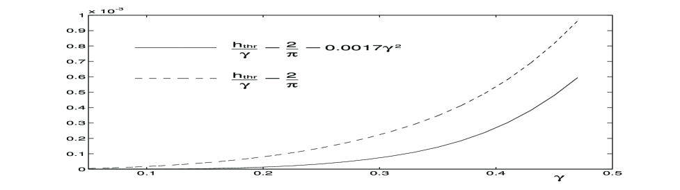
FIG. 1.: The comparison of the numerically obtained threshold values and their analytic approximations. Plotted is the difference $\left(h_{{\rm thr\/}(numerical)}-h_{{\rm thr\/}(analytic)}\right)/\gamma$, where $h_{{\rm thr\/}(analytic)}$ is given by $(2/\pi)\gamma$ (dashed curve) and $(2/\pi)\gamma+0.0017\gamma^{3}$ (solid line).

IV A unified viewpoint

The singular expansion of the previous section was designed as a continuation and generalization of the regular expansion and presented in the form that allows for a straightforward comparison with the latter. A natural step now is to try to develop a unified approach which would be valid both near and far from the turning point. Such a unified formalism could provide an additional insight into the structure of solutions and have some technical advantages.

The unification is achieved if one notices that the role of the coefficients $A,B,...$ is simply to renormalize the constant phase of the leading-order approximation $\psi_{0}=i{\rm sech\/}x$. Consequently, instead of adding homogeneous solutions $A{\rm sech\/}x$, $B{\rm sech\/}x,...$ at each order of $\gamma$ we can expand $\alpha$:

$$\alpha=\alpha_{0}+\alpha_{1}\gamma+\alpha_{2}\gamma^{2}+....$$ (59)

(This observation belongs to D. E. Pelinovsky.) Multiplying Eq.(3) through by $e^{i\alpha}$:

$$\psi_{xx}+2|\psi|^{2}\psi-\psi=-i\gamma\psi-he^{i\alpha},$$ (60)

and substituting Eqs.(45), (59) and (6) with $u_{0}=0$ and $v_{0}={\rm sech\/}x$, we get, at the order $\gamma$:

$${\mathfrak{h}}_{0}=\frac{2}{\pi}\frac{1}{\cos{\alpha_{0}}};$$ (61)

$$u_{1}={\cal U}_{1},\quad v_{1}={\mathfrak{h}}_{0}\sin\alpha_{0}L_{1}^{-1}1,$$ (62)

with ${\cal U}_{1}$ as in Eq.(33). For any $\alpha_{0}$ Eq.(61) gives the initial slope of the curve $h(\gamma)$ along which we want to continue our solution. The lowest $h$ arises for $\alpha_{0}=0$; hence in order to obtain the threshold one has to set ${\mathfrak{h}}_{0}=2/\pi$. Next, the order $\gamma^{2}$ yields

$${\mathfrak{h}}_{1}={\mathfrak{h}}_{0}\tan\alpha_{0}\left\{\alpha_{1}+\frac{1}{\pi}\int v_{0}(1-4v_{0}u_{1})L_{1}^{-1}1dx\right\}$$ (63)

and

$$v_{2}=L_{1}^{-1}(u_{1}+2v_{0}u_{1}^{2}+{\mathfrak{h}}_{0}\alpha_{1}).$$ (64)

Eq.(63) relates ${\mathfrak{h}}_{1}$ and $\alpha_{1}$. One of these (say, ${\mathfrak{h}}_{1}$) can be chosen freely; then Eq.(63) fixes the other. This simply means that given a nonzero $\alpha_{0}$, the solution exists for an arbitrary ${\mathfrak{h}}_{1}$ (i.e. in an arbitrary neighbourhood of the ray $h={\mathfrak{h}}_{0}\gamma$.) The case $\alpha_{0}=0$ is exceptional; in this case the ray is very close to the threshold and so we have to set ${\mathfrak{h}}_{1}=0$ while $\alpha_{1}$ remains undetermined. (This is the case where we would have to invoke the singular expansion before.) The coefficient $\alpha_{1}$ can only be fixed at the $\gamma^{3}$-level, where we obtain

$$\frac{1}{\pi}\int v_{0}\left\{2[u_{1}(u_{1}^{2}+v_{1}^{2})+2v_{0}(u_{1}v_{2}+u_{2}v_{1})]-v_{2}\right\}dx=$$

$$={\mathfrak{h}}_{1}\alpha_{1}\sin\alpha_{0}-{\mathfrak{h}}_{2}\cos\alpha_{0}+{\mathfrak{h}}_{0}\left(\alpha_{2}\sin\alpha_{0}+\frac{\alpha_{1}^{2}}{2}\cos\alpha_{0}\right).$$

Letting $\alpha_{0}=0$ this becomes exactly the quadratic equation (48) (where we only need to replace $A\to\alpha_{1}$) and hence we have reproduced our previous threshold.

Note that in the new formalism the corrections in the phase of $\psi_{0}$ are uncoupled from the rest of the expansion. The advantage of this is that the correction $\alpha_{1}$ ($=A$ in the previous notation) arises at the order $\gamma^{2}$ and not at $O(\gamma)$ as before; the correction $\alpha_{2}$ (previously known as $B$) arises at $O(\gamma^{3})$ and not at $O(\gamma^{2})$, and so forth. As a result, $u_{1}$ does not contain the unknown $\alpha_{1}$ ($A$); the correction $v_{2}$ depends on $\alpha_{1}$ only linearly (not quadratically as before), and so the resulting equation for $\alpha_{1}$ is manifestly quadratic. (Recall that Eq.(48) arises initially as a cubic equation and only then the coefficient of the term $A^{3}$ is calculated to be zero.)

V Concluding remarks and conclusions

1. In the undamped case ($\gamma=0$) for any $h\in(0,\sqrt{2/27})$ Eq.(3) has two explicit solutions [10]:

$$\psi^{(\pm)}(x)=\psi_{\infty}\left\{1+\frac{2\sinh^{2}\beta}{1\pm\cosh({\cal A}x)\cosh\beta}\right\},$$ (65)

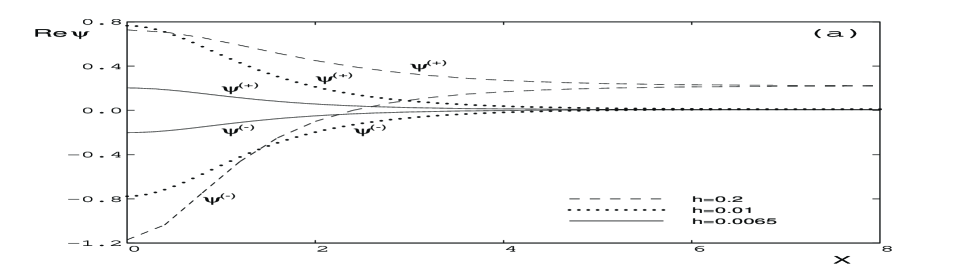
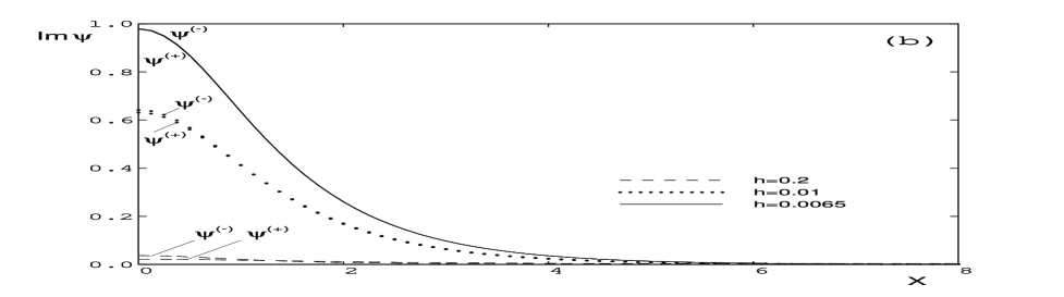
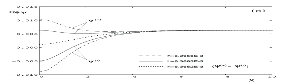
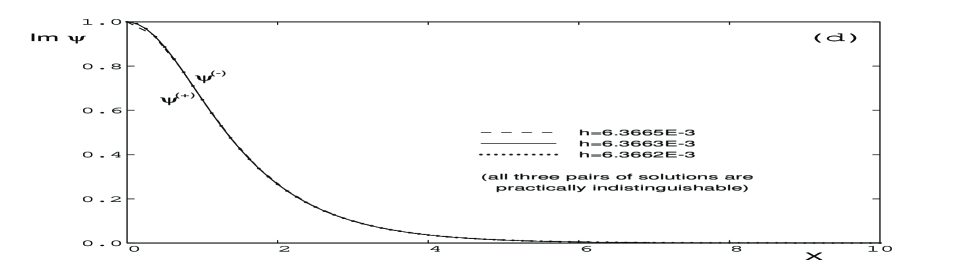
FIG. 2.: Soliton transformation for small $\gamma$ ($\gamma=0.01$). (a,b): For $h$ far above the turning point $h_{\rm thr}=6.3661997\times 10^{-3}$ the imaginary parts are close to zero and the two solitons are well approximated by the two undamped solitons (65) (dashed lines). As $h$ approaches the turning point, the real parts decrease and converge while imaginary parts grow (dotted then solid lines.) (c,d): In the immediate vicinity of $h_{\rm thr}$ the hump in the $\psi^{(+)}$ profile rapidly transforms into a dip and the two solitons collapse into one (dashed then solid then dotted line.) All functions being even, we only show them for positive $x$.

where

$$\psi_{\infty}=\left\{2(1+2\cosh^{2}\beta)\right\}^{-1/2}$$

is the asymptotic value of $\psi^{(\pm)}(x)$ as $|x|\to\infty$; the parameter $\beta$ is defined by inverting the relation

$$h=\frac{\sqrt{2}\cosh^{2}\beta}{(1+2\cosh^{2}\beta)^{3/2}},$$

and ${\cal A}$ is given by

$${\cal A}=2\psi_{\infty}\sinh\beta=\frac{\sqrt{2}\sinh\beta}{\sqrt{1+2\cosh^{2}\beta}}.$$

For the given value of $h$ the $\psi^{(+)}$ branch merges with $\psi^{(-)}$ at some $\gamma_{\rm thr}$ [defined, approximately, by $h=(2/\pi)\gamma_{\rm thr}+{\mathfrak{h}}_{2}^{(0)}\gamma_{\rm thr}^{3}$]. If $h$ is small then this $\gamma_{\rm thr}$ is also small, so that the point of the merger is very close to the $h$-axis and hence intuitively one could expect solutions at this point to be close to the undamped solitons (65). However, it is not quite obvious how this proximity can be reconciled with the fact that the two real solutions (65) are rather far from each other.

A related question concerns the shape of the $\psi^{(+)}$ and $\psi^{(-)}$ solitons. In the undamped case [Eq.(65)] the real function $\psi^{(+)}$ has a hump and $\psi^{(-)}$ has a dip. The numerical analysis shows that the hump respectively the dip persist in real parts of $\psi^{(+)}$ respectively $\psi^{(-)}$ solitons for $\gamma\neq 0$ [12]. Again, it is intuitively not quite obvious how the hump can transform into dip as the two branches merge. Shall this transformation proceed via the flat state?

The behaviour of solutions for small $h$ and $\gamma$ (in particular, near the turning point) can be clarified by invoking the asymptotic expansions (II) and (III). For the sake of illustration, we have also computed the two solitons numerically for a fixed small $\gamma$ ($\gamma=0.01$) and varying $h$; results are shown in Fig.2. In agreement with Eq.(II), for not very small $h$ ($h\gtrsim 0.1$) the imaginary parts of the solitons are seen to be almost zero [dashed lines in Fig.2(b)] while the real parts change slowly with the variation of $h$. For these $h$ the pair of real solutions (65) does indeed provide a good approximation for the corresponding $\psi^{(\pm)}$ with $\gamma=0.01$. However, as $h$ goes down, the real parts start changing (decreasing in magnitude) more vigorously while the imaginary parts are not small any longer; consequently, the approximation deteriorates. Near the turning point the real parts of both solitons become much smaller than their imaginary parts [see Fig. 2(c,d)]. Nevertheless, for $h$ not very close to the turning point (more specifically, for $h\geq 6.3665\times 10^{-3}$), the real part of $\psi^{(+)}$ still has a hump and real part of $\psi^{(-)}$ still has a dip [Fig. 2(a)]. This justifies our usage of the notations $\psi^{(+)}$ and $\psi^{(-)}$ for $\gamma\neq 0$. Finally, in a very near vicinity of the existence threshold $h_{\rm thr}=6.3662\times 10^{-3}$, the hump of the real part quickly transforms into the dip [Fig.2(c)].

This rapid change near the turning point can be easily understood in terms of the singular expansion (III). When ${\mathfrak{h}}_{2}$ is close to ${\mathfrak{h}}_{2}^{(0)}$, we can define a small $\epsilon$ by writing

$$\pi{\mathfrak{h}}_{2}=\pi{\mathfrak{h}}_{2}^{(0)}+\epsilon.$$ (66)

The corresponding $A$’s in Eq.(31) are then given by

$$A^{(\pm)}=A^{(0)}\pm\sqrt{\epsilon}.$$ (67)

Recalling that to the leading order in $\gamma$ it is only this coefficient $A$ that determines the dependence of solutions on $h$, Eq.(67) gives the rate of change of their real parts:

$$\frac{\partial u}{\partial{\mathfrak{h}}_{2}}=\pm\frac{\pi}{2}\frac{\gamma}{\sqrt{\epsilon}}\,{\rm sech\/}x+O(\gamma^{2}).$$ (68)

As $\epsilon\to 0$, the rate of change becomes infinitely large. Away from the neighbourhood of the turning point, in the region of the applicability of the regular expansion (II), the rate of the transformation of the solitons $\psi_{\pm}$ is given by

$$\frac{d\alpha}{d{\mathfrak{h}}}=\frac{2}{\pi{\mathfrak{h}}}\frac{1}{\sqrt{{\mathfrak{h}}^{2}-(2/\pi)^{2}}}.$$

Similarly to Eq.(68), this shows that as ${\mathfrak{h}}\to 2/\pi$, the two solitons transform increasingly fast.

Thus if we want to use the two real solitons (65) as approximations for their respective ($\gamma\neq 0$)-counterparts, we should keep in mind that this approximation is valid only far away from the turning point $\gamma_{\rm thr}$. Since for small $h$ the turning point is close to the $h$-axis (i.e. $\gamma_{\rm thr}\sim(\pi/2)h$ is also small), the validity of the approximation will be restricted to very small $\gamma$: $\gamma/h\ll\pi/2$.

2. Finally, we briefly summarize the main points of this work.

(a.) The lower boundary of the existence domain of the two solitons is given by the following asymptotic expression (as $\gamma\to 0$):

$$h_{\rm thr}=\frac{2}{\pi}\gamma+(1.667\times 10^{-3})\gamma^{3}+....$$ (69)

(b.) For $h$ away from the above threshold, more precisely for $h-(2/\pi)\gamma\gg 0.002\gamma^{3}$, the solitons are given by the asymptotic expansion Eq.(II) where $v_{1}$ and $u_{1}$ are given by explicit expressions (29)-(29) with $A^{(0)}=-2.4378\times 10^{-1}$.

(c.) For $h$ close to the turning point, $h=(2/\pi)\gamma+{\mathfrak{h}}_{2}\gamma^{3}$ with ${\mathfrak{h}}_{2}\sim 10^{-3}$ the second, $\gamma^{2}$-order of the regular expansion (II) becomes greater than the first order, and the expansion breaks down. In this case the two solitons are given by the singular expansion (58) with $A^{(\pm)}$ as in Eq.(53) and ${\mathfrak{h}}_{2}^{(0)}=1.667\times 10^{-3}$.

VI Acknowledgments

We thank Dmitry Pelinovsky for reading the manuscript and making a useful suggestion (which gave rise to the unified formalism of Sec.IV). Michael Kollmann’s and Mikhail Bogdan’s remarks and Nora Alexeeva’s computational assistance are also highly appreciated. I.B. is grateful to George Tsironis, Theo Tomaras and Nikos Flytzanis for their hospitality at the University of Crete. This research was supported by the FRD of South Africa and the URC of the University of Cape Town. I.B. was also supported by the FORTH of Greece and E.Z. was supported by an RFFR grant $\#$RFFR 97-01-01040.

REFERENCES

- [1] On sabbatical leave from Department of Mathematics, University of Cape Town, Rondebosch 7701, South Africa. Electronic address: igor@maths.uct.ac.za
- [2] Electronic address: zemel@cv.jinr.ru
- [3] L. A. Lugiato and R. Lefever, Phys. Rev. Lett. 58, 2209 (1987); M. Haeltermann, S. Trillo and S. Wabnitz, Opt. Lett. 17, 745 (1992); Opt. Commun. 91, 401 (1992); S. Wabnitz, Opt. Lett. 18, 601 (1993)
- [4] E. B. Volzhan, N. P. Giorgadze, and A. D. Pataraya, Fizika Tverdogo Tela, 18, 2546 (1976) [Sov. Phys. Solid State, 18, 1487 (1976)]; M. M. Bogdan, PhD thesis, FTINT, Kharkov (1983); G. Wysin and A. R. Bishop, J. Magnetism and Magnet. Materials 54-57, 1132 (1986); G. A. Maugin and A. Miled, Phys. Rev. B 33, 4830 (1986); A. M. Kosevich, B. A. Ivanov and A. S. Kovalev, Phys. Rep. 194, 118 (1990)
- [5] G. J. Morales and Y. C. Lee, Phys. Rev. Lett. 33, 1016 (1974); A. V. Galeev, R. Z. Sagdeev, Yu. S. Sigov, V. D. Shapiro and V. I. Shevchenko, Fiz. Plazmy, 1, 10 (1975) [Sov. J. Plasma Phys. 1, 5 (1975)]
- [6] K. Maki, Phys. Rev. B 18, 1641 (1978); D. J. Kaup and A. C. Newell, Phys. Rev. B 18, 5162 (1978); D. Bennett, A. R. Bishop and S. E. Trullinger, Z. Phys. B 47, 265 (1982)
- [7] Lei Lin, C. Shu and G. Xu, J. Stat. Phys. 39, 633 (1985)
- [8] D. W. McLaughlin and A. C. Scott, Phys. Rev. A 18, 1652 (1978); J. C. Eilbeck, P. S. Lomdahl and A. C. Newell, Phys. Lett. A 87, 1 (1981); M. Salerno and A. C. Scott, Phys. Rev. B 26, 2474 (1982); F. If, P. L. Christiansen, R. D. Parmentier, O. Skovgaard, and M. P. Soerensen, Phys. Rev. B 32, 1512 (1985); M. Fordsmand, P. L. Christiansen, and F. If, Phys. Lett. A 116, 71 (1986)
- [9] Y. Braiman, W. L. Ditto, K. Wiesenfeld and M. L. Spano, Phys. Lett. A 206, 54 (1995); Y. Braiman, J. F. Lindner and W. L. Ditto, Nature 378, 465 (1995); L. M. Floria and J. J. Mazo, Adv. Phys. 45, 505 (1996); A. Gavrielides, T. Kottos, V. Kovanis and G. P. Tsironis, Phys. Rev. E 58, No.5 (1998)
- [10] I. V. Barashenkov, M. M. Bogdan and T. Zhanlav, in Nonlinear World, Proceedings of the Fourth International Workshop on Nonlinear and Turbulent Processes in Physics, Kiev, 1989, edited by V. G. Bar’yakhtar et al. (World Scientific, Singapore, 1990), p.3.
- [11] G. Terrones, D.W. McLaughlin, E.A. Overman and A. Pearlstein, SIAM J. Appl. Math. 50, 791 (1990)
- [12] I.V. Barashenkov and Yu.S. Smirnov, Phys. Rev. E 54, 5707 (1996)
- [13] D. J. Kaup and A. C. Newell, Proc. Roy. Soc. London Ser. A 361, 413 (1978)
- [14] K. H. Spatschek, H. Pietsch, E. W. Laedke, and Th. Eickermann, in Singular Behaviour and Nonlinear Dynamics, Proceedings of International Conference, Samos, 1988, edited by St. Pnevmatikos, T. Bountis and Sp. Pnevmatikos. (World Scientific, Singapore, 1989), p.555
- [15] There is also an upper boundary; see [12] and I.V. Barashenkov, Yu.S. Smirnov and N.A. Alexeeva, Phys. Rev. E 57, 2350 (1998). The upper boundary arises due to bifurcations of a different type and requires an entirely different asymptotic formalism. We do not dwell on this in the present work.
- [16] M. Kollmann, H. W. Capel and T. Bountis. Breathers and multibreathers in a periodically driven damped discrete nonlinear Schrödinger equation. Preprint of Universiteit van Amsterdam, 1998; to appear in Phys. Rev. E.