Finger Competition and Formation of a Single Saffman-Taylor Finger without Surface Tension: An Exact Result

Abstract

We study the exact non-singular zero-surface tension solutions of the Saffman-Taylor problem [Mineev-Weinstein and Dawson, Phys. Rev. E 50, R24 (1994); Dawson and Mineev-Weinstein, Physica D 73, 373 (1994)] for all times. We show that all moving logarithmic singularities $a_{k}(t)$ in the complex plane $\omega=e^{i\phi}$, where $\phi$ is the stream function, are repelled from the origin, attracted to the unit circle and eventually coalesce. This pole evolution describes essentially all the dynamical features of viscous fingering in the Hele-Shaw cell observed by Saffman and Taylor [Proc. R. Soc. A 245, 312 (1958)], namely tip-splitting, multi-finger competition, inverse cascade, and subsequent formation of a single Saffman-Taylor finger.

Saffman-Taylor experiment. In 1958 Saffman and Taylor [1] studied the displacement of oil by water in a narrow gap between two parallel plates (the Hele-Shaw cell [2]). The three upper pictures in Fig.1 show three consecutive stages in their observations: initial, intermediate, and asymptotic. The small ripples in the left-most picture are caused by an instability of the initially almost planar oil/water interface. We call this initial stage perturbative since the deviation from a flat front is small, so the dynamics can be examined by perturbation theory [3]. Later, at the intermediate stage shown in the center picture, many fingers are formed along the moving interface. They compete, some are screened and then stagnate, some continue to advance and fatten, while new ones continue to appear because of tip-splitting. We call this second (intermediate) stage non-perturbative, since the deviation of the front from a straight line is no longer small and thus it cannot be studied perturbatively. Eventually, in the final asymptotic stage (the right picture), a single uniformly advancing finger dominates after all others are suppressed in the competition described above. This single finger occupies one half of the Hele-Shaw cell width $w$ and is described by the formula

$$x=2t+{\rm log}\,(\cos y)$$ (1)

where $w=2\pi$ in our scaled units; the longitudinal extent, that is the $x$-direction, is taken to be infinitely large; and velocities of both fluids are chosen to be 1 when $|x|~{}\rightarrow~{}\infty$. Throughout the last 40 years after [1] was published, this experiment has been reproduced many times, both in laboratories and by numerical calculations. (See [4] and references therein). The process above was found to be universal and independent of the specific liquids (oil and water in [1]) provided the fluids are immiscible and incompressible and a driving fluid is much less viscous than a driven one.

A mathematical formulation in the absence of surface tension and in scaled units is

$$\nabla^{2}p=0\quad{\rm(in~{}the\,oil~{}domain)}$$ (2)

$$p=-x\quad{\rm if}~{}~{}x\,\to+\infty\,\quad{\rm(oil~{}pushed~{}to~{}the~{}right)}$$ (3)

$$p=0\quad{\rm(at~{}the~{}oil/water~{}interface)}$$ (4)

$$\partial_{n}p=0\quad{\rm for}~{}~{}y=\pm\pi\,\quad\rm{(at~{}the~{}channel~{}walls)}$$ (5)

$$V_{n}=-\partial_{n}p\quad\rm{(at~{}the~{}oil/water~{}interface)}$$ (6)

where $V_{n}$ is the normal velocity of the interface, $p$ is pressure, and $\partial_{n}$ is the normal derivative. From (2) follows the Laplacian growth equation (LGE) (see [5] and references therein), which can be written compactly as:

$${\rm Im}(\bar{z}_{t}z_{\phi})=1\,\,,$$ (7)

for the moving front $z(t,\phi)=x(t,\phi)+iy(t,\phi)$, parameterized by $\phi\in[0,2\pi]$. Here the bar denotes the complex conjugate; $z_{t}$ and $z_{\phi}$ are partial derivatives; and the map $\phi\rightarrow z(t,\phi)$ is conformal for Im $\phi\leq 0$.

Derivation of the LGE (3) from (2) follows. Because of the identity $V_{n}={\rm Im}(\bar{z}_{t}z_{l})$, where $l$ is an arclength along the front, and of the Cauchy-Riemann relation, $-\partial_{n}p~{}=~{}\partial_{l}\phi$ for pressure $p$ and stream function $\phi$, where $\partial_{l}$ is the tangential derivative, the last equation in the system (2) can be rewritten as

$${\rm Im}(\bar{z}_{t}z_{l})=\partial_{l}\phi$$

which is equivalent to (3); ($\partial_{l}\phi=-\partial_{n}\,p\neq 0$, since $p=0$ along the front and because of the maximum principle for harmonic functions). It then follows that the variable $\phi$ in (3) is the stream function. The map $\phi\rightarrow z(t,\phi)$ is conformal for Im $\phi\leq 0$, since the complex velocity potential $W(z)=-p(x,y)+i\phi(x,y)$ is analytic in the oil domain.

Previous studies have focused primarily on the selection of the asymptotic finger width $\lambda$ from the continuous family, found in [1]:

$$x=\frac{t}{\lambda}+2(1-\lambda)\,{\rm log}(\cos\frac{y}{2\lambda})$$ (8)

where the finger moves to the right with velocity $1/\lambda$, and the finger’s dimensionless width $\lambda$, measured in units of the channel width, can be any number between $0$ and $1$. (It is not difficult to see that (4) is the traveling-wave solution of (3)). These selection studies focused on surface tension as the critical factor, which determines the finger width $\lambda$ [4,6]. (When $\lambda=1/2$, (4) becomes (1)). Some studies (mostly numerical and semi-analytical) also addressed the intermediate (non-perturbative) period of the process [7], and again, as in the case of width selection, all the main features observed during this stage were attributed to non-zero surface tension. We believe that this attitude was formed because almost all exact solutions known at that time [8] for zero surface tension exhibited finite-time singularities (cusps). The inevitability of cusps was related to the ill-posedness of the problem in the absence of surface tension [10]. Recently however the selection of $\lambda=1/2$ was solved [11] in the absence of surface tension using the exact time-dependent $N$-logarithmic solutions of the LGE (3), which remain non-singular and analytic for all time (no cusps)[5].

These N-logarithmic solutions have the form [5]:

$$z(t,\phi)=\tau(t)+i\mu\phi+\sum_{k=1}^{N}\alpha_{k}\log(e^{i\phi}-a_{k}(t))\,,$$ (9)

where $\alpha_{k}={\rm const}$, $|a_{k}|<1$, $\mu=1-\sum_{k=1}^{N}\alpha_{k}$, and $\mu\in[-1,1]$. With some constraints on $\{\alpha_{k}\}$, which are not specified here (see [12] for details), these solutions remain regular and do not exhibit finite-time singularities [5], unlike all other known time-dependent solutions of (3). The time dependence of $a_{k}(t)$ and $\tau(t)$ is given by

$$\beta_{k}=\tau-\log\bar{a}_{k}+\sum_{l=1}^{N}\alpha_{l}\log(1-\bar{a}_{k}a_{l})=\rm{const}$$ (10)

$${\rm{and}}\,\,\,t+C=\tau+\frac{1}{2}\sum_{k=1}^{N}\sum_{l=1}^{N}\alpha_{k}\bar{\alpha}_{l}\log(1-a_{k}\bar{a}_{l})$$ (11)

where $C$ and $\beta_{k}$ ($k=1,2,...,N$) are constants in time. The validity of (6) and (7) can be easily verified after substitution of (5) into (3) [13]. The solutions (5) are dense in the space of analytic curves [14], and all singularities of $z_{\phi}$ are simple poles $a_{k}(t)$, while all other known solutions of (3) [8] have multiple poles. Thus (5) are the most natural and generic exact solutions of (3) with a finite number of moving singularities.

The geometrical interpretation of (5) is of great help (see Figure 2): The constant of motion $\beta_{k}-\alpha_{k}\log 2$ is also the complex coordinate of the stagnation point at the vertex of the $k^{th}$ “groove” with parallel walls. This groove originates during the front evolution; $\pi|\alpha_{k}|$ is the width of this groove, and arg($\alpha_{k}$) is the angle between the axis of symmetry of the groove and the horizontal axis. This interpretation of solutions (5) is in excellent agreement with all known low surface tension experiments; and we claim that all stages of this process are faithfully described by (5) (to be more exact - appropriate subset of (5) [15]).

The goal of this paper is to show how the exact solution (5) describes essentially all stages of the Saffman-Taylor process, but especially formation of a single Saffman-Taylor finger. Incidentally, we also show how the zero-surface-tension solution (5) can reproduce the following dynamical phenomena observed in this process and attributed traditionally to surface tension: tip-splitting, side-branching, screening of retarded and coarsening of advanced fingers, and formation of a single finger after finger competition.

To accomplish our goal we will study the dynamical system of the poles $a_{k}(t)$ defined by (6-7) on the mathematical plane $\omega=e^{i\varphi}$. As mentioned above, the dynamics of poles $a_{k}$ provides, through (5), a complete description of these phenomena in the physical plane $z=x+iy$. In particular, the coalescence of all poles, which we prove below, explains why only a single finger survives in the long-time asymptotics. The pictures at the bottom of Fig.1 show typical distributions of singularities $a_{k}$ inside the unit circle associated with all three stages of this process.

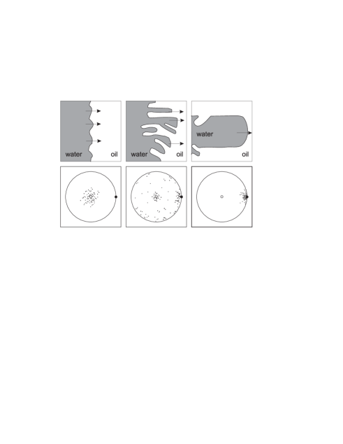
FIG. 1.: Three consecutive stages of viscous fingering in the Hele-Shaw cell: initial (left), intermediate (center), and asymptotic (right). The physical plane $z$ is shown in the upper pictures, while the lower pictures depict a distribution of moving poles $a_{k}(t)$ in the unit circle $|\omega|<1$ on the mathematical plane $\omega$. The open circle indicates the repeller, $\omega=0$, while the solid circle indicates the attractor, $\omega=1$, of poles whose dynamics is given by (6-7).

Initial stage: disordering begins, the repeller at $\omega=0$. For a front that is almost flat initially, all singularities are near the origin: $|a_{k}|\,\ll\,1$ (see the left of Fig.1). Indeed, in this case the front is almost planar: $z(0,\phi)\cong\tau+i\phi$. Then the singularities $a_{k}$ start to move away from the origin. One can easily see from (6) that, if $|a_{k}|\,\ll\,1$, $|a_{k}|\cong e^{\tau}$. This exponentially fast repulsion from the origin, holds for every pole $a_{k}$, if $|a_{k}|\,\ll\,1$, regardless of the positions of the other poles. It means that $\omega=0$ is the repeller for the dynamical system of $a_{k}(t)$ specified by (6) and (7). As one can easily see, $a_{k}=0$ is an unstable equilibrium solution of the dynamical system (6-7). (The corresponding $\beta_{k}$ equals infinity.) The repulsion from zero manifests itself in the front instability, which always occurs when a less viscous fluid pushes a more viscous one. Indeed, the closer $a_{k}$ comes to the unit circle, the more complex the interface becomes.

Because of the exponentially fast instability, the system quickly enters into the non-perturbative stage: convex parts of the interface accelerate, while concave parts decelerate, retard, eventually stagnate and start to form grooves near their most retarded points (stagnation points). The tendency of moving fronts to form these grooves with almost parallel walls has been observed in numerous laboratory and computational experiments [4,6,7]. The dynamics of formation of these grooves coincides with the dynamics of the solution (5), given by (6) and (7), near the points $z(t,\phi)\cong\beta_{k}-\alpha_{k}\log 2$ and is fully compatible with the geometrical interpretation of (5) given above. It is unknown, though, why these grooves have parallel (or almost parallel) walls.

Early intermediate stage: disordering increases. The formation of grooves near stagnation points explains such frequently observed dynamical features as tip-splitting and side-branching of the moving interface. Each such event makes the moving interface more complex: it increases the effective number of grooves by one, and consequently the total number of grooves grows in time. (One can equally say that the number of fingers grows in time, since a finger, as we traditionally call it, is an element of the advancing front between two adjacent grooves. Note that while grooves have parallel walls, fingers, as a rule, do not.) In short, disordering and complexity of the front increases during this stage (the center of Fig.1).

As shown in [5], the only long time asymptotics for each $a_{k}(t)$ consistent with (6) is $|a_{k}|\rightarrow 1$. This was shown assuming that Re$\,\alpha_{k}\geq 0$ for each $k=1,2,...,N$. This assumption was taken in [5] as a working criterion for the solutions (5) to be non-singular. Recent studies showed that this criterion is too simple [12], but for many scenarios it works successfully. Since (6) and (7) require all singularities $a_{k}(t)$ to move toward the unit circle (see details in [5]), they eventually enter its narrow vicinity and accumulate there. The $a_{k}$’s continue to approach the unit circumference $|\omega|=1$ exponentially slowly, namely as $1-|a_{k}|=c_{k}\exp{(-\tau/{\rm Re}\,\alpha_{k})}$, when $c_{k}>0$, Re $\alpha_{k}>0$, and when the poles $a_{k}$ are not too close to each other. Only when $a_{k}$ approaches the unit circle does the groove near the stagnation point $\beta_{k}-\alpha_{k}\log 2$ develop. In this sense the geometrical interpretation of the constants $\alpha_{k},\beta_{k}$ given above is applicable only in intermediate asymptotics, that is when $|a_{k}|$ approaches one.

Late intermediate stage: ordering begins. “The law of nonlinear superposition” for groove merging. It was indicated and discussed in [5,16] that when two poles $a_{k}$ are close to the unit circle, they are mutually attracted along the angular direction, cannot pass each other and must merge. This merging is complete only when $\tau\rightarrow\infty$, while for finite $\tau$, the distance between merged poles is, as one can see from (6), of the order of $e^{-b\tau}$, where $b>0$. As two poles merge, say $a_{1}$ and $a_{2}$, we equate them, so the total number of logarithmic terms in the sum in (5) decreases by one, and a new logarithmic term in this sum forms from the two terms labeled by $1$ and $2$. The coefficient of this new term clearly is $\alpha_{1}+\alpha_{2}$. In the physical plane this corresponds to the merging of two grooves into a single one. The width and the angle (to the horizontal axis) of the newly formed groove are $\pi|\alpha_{1}+\alpha_{2}|$ and $\arg(\alpha_{1}+\alpha_{2})$ respectively, while the widths and angles of two grooves before their interaction were $\pi|\alpha_{1}|$, $\pi|\alpha_{2}|$ and $\arg\alpha_{1}$, $\arg\alpha_{2}$ respectively. An example is shown in Fig.2.

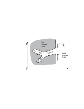
FIG. 2.: Geometrical interpretation of the complex constants of motion $\alpha_{k}$ and $\beta_{k}$; $k=1,...,N$.

This “law of non-linear superposition” of grooves governs the interaction between these grooves and determines all the dynamics of groove coalescence. Each interaction of this kind leaves one of interacting fingers behind, while the others continue to advance and fatten, thus “winning the competition”. Two adjacent fingers do not interact only if they are strictly parallel. Later we will show that this parallel configuration is linearly unstable. As a result of this merging the total number of advancing fingers is decreased by one. (Or, what is the same, the total number of effective grooves decreases by one after each pair coalescence). In this fashion, the solutions (5) describe the phenomenon of finger competition (or groove coalescence). This ordering process eventually dominates the disordering due to tip-splitting and side-branching (which is just the birth and development of new grooves). So, in the long-time asymptotics only a single finger is left to propagate (Fig.1 upper-right).

Physically, the merging of grooves is an inverse cascade, an ordering process that dominates after saturation. This self-organizing behavior of an unstable front is not exceptional: it occurs in several unstable nonlinear processes in confined geometries [17]. It is the walls of the box the system is contained in, which stabilize growth. This happens when the transverse correlation length, initially small, becomes comparable with the lateral width of the box [18]. Then in all these processes a universal pattern appears (different for different processes). In the dynamics described by (2), this pattern is the single finger, observed by Saffman and Taylor in [1].

The rest of this paper derives the coalescence of all singularities $a_{k}$ at a single point on the unit circle (for periodic boundary conditions at the walls) or at two opposite points on the unit circle $a_{k}\rightarrow\pm 1$ (for no-flux boundary conditions at the walls). In the physical plane, this means that, for generic initial data in the class of non-singular solutions (5), the asymptotics $t\rightarrow\infty$ is indeed a single uniformly advancing finger in accordance with experimental observations. Then replacing every $a_{k}$ by 1 and $\tau$ by $Vt$ in (5) when $t\rightarrow\infty$, we obtain

$$z(t,\varphi)=Vt+\mu i\varphi+(1-\mu)\log(e^{i\varphi}-1)$$

which coincides with (4) when $V=1/\lambda$ and $\mu=2\lambda-1$ and thus describes a single uniformly moving finger, as expected. (To select $\lambda=1/2$ within the class (5), it is sufficient to move the pole infinitesimally away from the unstable equilibrium that is zero, as was shown in [11].)

The variable $\tau$ is a scaled time. First we prove that $\tau$ in (5-7) is but a scaled time, and it will be treated as such below. First, we note that $d\tau/dt$ is always finite, since we consider only non-singular solutions (5). Then we see that always $\tau>t$. To prove this, we expand every logarithm in the RHS of (7) as an infinite power series. We obtain

$$t=\tau-\frac{1}{2}\sum_{m=1}^{\infty}\frac{|\sum_{k=1}^{N}\alpha_{k}a_{k}^{m}|^{2}}{m}$$

(setting $C=0$ in (7).) Thus $\tau>t$. Then if $t\,\rightarrow\,\infty$, so does $\tau$. It follows from (6) and (7) that

$$t+C^{\prime}=\frac{1+\mu}{2}\tau+\frac{1}{2}\sum_{k=1}^{N}\alpha_{k}\log(a_{k})$$ (12)

where $C^{\prime}$ is a constant. The only way to compensate the divergent positive term $\tau$ in the RHS of (6) is to admit that $|a_{k}|\,\rightarrow\,1$ for each $k=1,2,...,N$ [19].The only way to compensate the divergent positive term $\tau$ in the RHS of (6) is to admit that $|a_{k}|\,\rightarrow\,1$ for each $k=1,2,...,N$ [19]. Therefore in the long-time limit the relation between $t$ and $\tau$ is linear.

Proof that all poles coalesce in the long-time limit. We want to investigate the asymptotic behavior of the poles $a_{k}$ when $\tau\rightarrow\infty$. First, we introduce new variables $a_{k}=\exp\{-\eta_{k}+i\Phi_{k}\}$ and $\alpha_{k}=\alpha^{\prime}_{k}+i\alpha^{\prime\prime}_{k}$. The condition $|a_{k}|\rightarrow 1$ then simply means that $\eta_{k}\rightarrow 0+$. In order to eliminate the divergent term $\log(1-|a_{k}|^{2})$ from (6) we multiply (6) by $\bar{\alpha}_{k}$ and then extract its imaginary part. The result is

$${\rm Im}(\bar{\alpha}_{k}\beta_{k})=\alpha^{\prime}_{k}\Phi_{k}-\alpha^{\prime\prime}_{k}\tau$$ (13)

$$+\sum_{l\neq k}^{N}[(\alpha^{\prime\prime}_{l}\alpha^{\prime}_{k}-\alpha^{\prime\prime}_{k}\alpha^{\prime}_{l})\log|1-\bar{a}_{k}a_{l}|$$ (14)

$$+\,(\alpha^{\prime}_{k}\alpha^{\prime}_{l}+\alpha^{\prime\prime}_{l}\alpha^{\prime\prime}_{k})\,{\rm arg}(1-\bar{a}_{k}a_{l})].$$ (15)

(We neglected the small term, $-\alpha^{\prime\prime}_{k}\eta_{k}$). Here we have the divergent term $-\alpha^{\prime\prime}_{k}\tau$. To compensate this divergence we need to assume that at least some poles coalesce. That is $N$ poles $a_{k}$ are divided into $\tilde{N}$ groups of merging poles $a_{k}$ so that $|\Phi_{k}-\Phi_{l}|\rightarrow 0$ for all members of each group. After summation of eqs. (9) over all poles within each of the $\tilde{N}$ groups, we obtain

$$C_{m}=\tilde{\alpha}^{\prime}_{m}\tilde{\Phi}_{m}-\tilde{\alpha}^{\prime\prime}_{m}\tau$$ (16)

$$+\sum_{n\neq m}^{\tilde{N}}[(\tilde{\alpha}^{\prime\prime}_{n}\tilde{\alpha}^{\prime}_{m}-\tilde{\alpha}^{\prime\prime}_{m}\tilde{\alpha}^{\prime}_{n})\log|1-\bar{\tilde{a}_{m}}\tilde{a}_{n}|$$ (17)

$$+(\tilde{\alpha}^{\prime}_{m}\tilde{\alpha}^{\prime}_{n}+\tilde{\alpha}^{\prime\prime}_{m}\tilde{\alpha}^{\prime\prime}_{n})\,{\rm arg}(1-\bar{\tilde{a}_{m}}\tilde{a}_{n})]\,\,.$$ (18)

Here $C_{m}$ are constants, $\tilde{\Phi}_{m}=\arg\tilde{a}_{m},\,\tilde{\alpha}^{\prime}_{m}=\sum_{k=1}^{n_{m}}\alpha^{\prime}_{k}$,  $\tilde{\alpha}^{\prime\prime}_{m}=\sum_{k=1}^{n_{m}}\alpha^{\prime\prime}_{k}$, $n_{m}$ is the number of poles in the $m$-th group, and $1\,\leq\,m\,\leq\,\tilde{N}$. Also because of the partial merging, all poles within each group labeled by $m$ are equated to $\tilde{a}_{m}$ with an exponentially high accuracy. Replacing (with the same accuracy) $|\tilde{a}_{m}|$ by 1, and assuming no merging between different $\tilde{a}_{m}$’s, which means

$$|\Phi_{k}-\Phi_{l}|\gg\eta_{k}+\eta_{l}$$

where $k$ and $l$ are from different groups, we rewrite (10) as

$$C^{\prime}_{m}=\tilde{\alpha}^{\prime}_{m}\tilde{\Phi}_{m}-\tilde{\alpha}^{\prime\prime}_{m}\tau$$ (19)

$$+\sum_{n\neq m}^{\tilde{N}}[(\tilde{\alpha}^{\prime\prime}_{n}\tilde{\alpha}^{\prime}_{m}-\tilde{\alpha}^{\prime\prime}_{m}\tilde{\alpha}^{\prime}_{n})\log|\sin(\frac{\tilde{\Phi}_{m}-\tilde{\Phi}_{n}}{2})|$$ (20)

$$+(\tilde{\alpha}^{\prime}_{m}\tilde{\alpha}^{\prime}_{n}+\tilde{\alpha}^{\prime\prime}_{n}\tilde{\alpha}^{\prime\prime}_{m})\frac{\tilde{\Phi}_{n}-\tilde{\Phi}_{m}}{2}],$$ (21)

where $C^{\prime}_{m}$ are new constants. From this equation we conclude that

(i) Since $\log|\sin(\frac{\tilde{\Phi}_{m}-\tilde{\Phi}_{n}}{2})|\rightarrow-\infty$ for $|\tilde{\Phi}_{m}-\tilde{\Phi}_{n}|\,\rightarrow 0,2\pi$, the poles cannot pass each other.

(ii) After summation over all $m=1,...,\tilde{N}$, we see that $\sum_{m}\tilde{\alpha}^{\prime}_{m}\tilde{\Phi}_{m}={\rm const}$.

(iii) From (i) it follows that once $0<\tilde{\Phi}_{m}-\tilde{\Phi}_{n}<2\pi$ in the long-time asymptotics it will hold for all further times.

(iv) From (ii) and (iii) it follows that $|\tilde{\Phi}_{m}|\rightarrow\infty$ is impossible.

(v) From (iii) and (iv) it follows that there is no way to compensate the divergent term $-\tilde{\alpha}^{\prime\prime}_{m}\tau$ in (11), except to admit that $\tilde{\alpha}^{\prime\prime}_{m}\,=\,0$ for each $l=1,...,\tilde{N}$.

Finally we conclude that

$$\tilde{\alpha}^{\prime\prime}_{m}=\sum_{j=1}^{n_{m}}\,\alpha^{\prime\prime}_{j}=0,\,\,\,\,\dot{\tilde{\Phi}_{m}}=0,\,\,\,\,\tilde{\Phi}_{m}\neq\tilde{\Phi}_{n}\,({\rm for}\,m\neq n)$$

To find the asymptotic motion of poles within each group containing $n_{m}$ poles we differentiate the equations (7) keeping only leading (divergent) terms:

$$\dot{\tau}\,+\,\sum_{l=1}^{n_{m}}\alpha_{l}\frac{\dot{\eta}_{l}+\dot{\eta}_{k}+i(\dot{\Phi}_{k}-\dot{\Phi}_{l})}{\eta_{l}+\eta_{k}+i(\Phi_{k}-\Phi_{l})}=0$$

The solution of these equations is

$$\eta_{k}=\eta_{k}^{0}e^{-\tau/\tilde{\alpha}^{\prime}_{m}}$$ (22)

$$\Phi_{k}-\Phi_{l}=(\Phi_{k}^{0}-\Phi_{l}^{0})e^{-\tau/\tilde{\alpha}^{\prime}_{m}}$$ (23)

provided that

$$\tilde{\alpha}^{\prime\prime}_{m}=\sum_{k=1}^{n_{m}}\,\alpha^{\prime\prime}_{k}=0.$$ (24)

Instability of configurations with two or more parallel fingers. Therefore, the only case when merging will not be complete occurs when two or more groups of sums of $\alpha_{k}$’s, that are $\tilde{\alpha}_{m}$’s, are real. This corresponds to the case (see the geometrical interpretation of $\alpha$’s above) when all newly formed grooves characterized by $\tilde{\alpha}_{m}$’s are parallel to each other (and to the horizontal axis). In this case instead of a single finger in the asymptotics, we would have several parallel fingers with grooves between them having widths of $\pi\,|\tilde{\alpha}_{m}|$. But this configuration is unstable: In order to verify this, let us perturb slightly the constants $\alpha^{\prime\prime}_{k}$ so that (12) is violated for every $m=1,\ldots,\tilde{N}$, or we may merely add new logarithmic terms to the sum in (6). Once we destroy (even slightly) the parallelism of the newly formed grooves that are partial sums of $\alpha_{k}$’s, then in accordance with the analysis above we have only one group of poles which satisfy (12). And this group contains all poles, so $\tilde{N}=1$. Hence we have total coalescence of all poles $a_{k}$. In the physical plane this means merging into a single groove (or, what is the same, a front forms a single finger).

The unique solution for $t\rightarrow\infty$ for each pole is

$$\eta_{k}=\eta_{k}^{0}e^{-2t/(1-\mu^{2})}$$ (25)

$$\Phi_{k}=\Phi_{k}^{0}e^{-2t/(1-\mu^{2})}$$ (26)

$$1-\mu^{2}>0$$ (27)

Here we used from (8) that $(1+\mu)\tau=2t$ for $t\rightarrow\infty$. Thus for periodic boundary conditions all poles $a_{k}$ coalesce at a single point on the unit circle (chosen to be $\omega=1$ in Fig.1). In the case of no-flux boundary conditions, which impose double periodicity with reflectional symmetry on this problem [11] (see also [20]), there are clearly two groups of poles mutually complex conjugate to each other. Because of this (mirror) symmetry, the attractors are real, and there are clearly two of them, $\omega=\pm 1$, in this case, instead of one attractor as for periodic boundary conditions.

Proof of total coalescence without any formulae. After the detailed analysis (10)-(13) leading to the necessity of total coalescence, we will show how to prove the main result of this paper without a single formula, by using only the geometrical interpretation of (5) and the “law of non-linear superposition” given above: Any two adjacent grooves whose axes of symmetry are not strictly parallel (which is clearly the generic case) will eventually coalesce. This will happen where their axes of symmetry cross. In accordance with Euclid, two non-parallel straight lines on the plane necessarily cross, and since each crossing means the coalescence of two grooves, eventually all grooves coalesce. At first glance, this proof is valid only for those grooves whose axes of symmetry cross in advance of the moving front, and invalid when they cross behind it. But the proof still works because of the mirror symmetry imposed by no-flux boundary conditions (see [11]). This implies that if the middle lines of two adjacent grooves cross behind the front, then one middle line and the mirror image of the other one necessarily cross in front of the interface, so again coalescence is unavoidable.

Summary of the asymptotic stage. After a cascade of subsequent groove crossings and coalescence, new grooves will be formed, described by $\tilde{\alpha}_{m}$, which are sums of the $\alpha_{k}$’s of the original grooves participating in coalescence. New grooves will coalesce by the same rules as the original ones, that is when their symmetry axes cross. Since the parallel configuration of two or several grooves is unstable, eventually a single groove will be formed with a width of $\pi(1-\mu)$. Since this is a real number, this final single groove will be parallel to the Hele-Shaw channel’s walls. Then the single finger (a moving front between two grooves) will propagate along the Hele-Shaw cell in accordance with observations. The finger width is $2\pi-\pi(1-\mu)=\pi(1+\mu)$, and the relative finger width measured in units of Hele-Shaw cell (chosen here to be $2\pi$) is $\lambda=\pi(1+\mu)/(2\pi)=(1+\mu)/2$. Regarding the selection of $\lambda=1/2$ from this family (that is, $\mu=0$) we will just repeat here the essence of [11], where two observations were made: that the origin is a point of unstable equilibrium (the repeller) for singularities, and that all fingers with a width different from one half correspond to the case when one of the singularities lies at the origin. Once this singularity is perturbed (released from zero), it moves with the rest of poles toward the attractor lying on the unit circle [11]. Then, once there are no singularities at zero, the asymptotic finger has a width $\lambda=1/2$, in accordance with experiments [1,4].

General summary. The solutions (5) indeed explain all stages of front dynamics in the Hele-Shaw cell in great detail. On the mathematical plane, the singularities $a_{k}$ move away from the repeller at the origin, where most of them are initially located, toward the unit circle which is the intermediate attractor for the dynamical system (6,7). On the physical plane this is a process of disordering which occurs in agreement with the geometrical interpretation, that is through the formation of grooves described by constants $\{\alpha_{k},\,\beta_{k}\}$, until the saturation time marks the end of the disordering part of the process. Then the system enters into the ordering part, when the number of competing fingers eventually decreases and finally a single finger survives the competition and persists to advance in the long-time asymptotic limit (Fig.1 upper-right). On the mathematical plane it means that when the radial component of poles’ velocities becomes small near the unit circle, the angular component brings pairs of singularities together, and they attract and coalesce. Then groups of coalesced singularities move as units near the unit circle and eventually merge together at a single point on the unit circle ($\omega=1$ in Fig.1), which is the only attractor in periodic boundary conditions. The no-flux boundary conditions imposing the reflectional symmetry make two attractors at $\pm 1$.

Conclusion. We have shown that the front expressed by non-singular solutions (5), which describe Laplacian growth in the Hele-Shaw cell in the absence of surface tension, forms a single finger uniformly propagating along the Hele-Shaw cell asymptotically in time. Essentially all the observed dynamical features of tip-splitting, finger competition, screening, coarsening, and finally forming a single finger are shown to be consequences of the solution (5) for a generic choice of initial parameters.

What is unclear. Here we mention questions for further elucidation: We have studied the asymptotics far beyond the farthest stagnation point $\beta_{k}$, implying that for some reason perturbations of the front eventually stop. What physically happens is that during the formation of the single finger, the front gradually stabilizes and eventually is no longer vulnerable to weak noise. Clearly, this stabilization cannot be justified without non-zero surface tension. It is remarkable that the zero surface tension solution (5) nevertheless works and explains all these phenomena including tip-splitting, side-branching, finger competition, screening and coarsening [5], formation of a single finger (the present paper), and the selection of its width of one half [11], in accordance with numerous observations. Why does it work without surface tension? And how does surface tension regulate population and location of stagnation points and width of grooves? The answers to these questions are not known today.

Acknowledgement. We gratefully acknowledge discussions with G. D. Doolen, J. Pearson, and I. Procaccia. We also appreciate help of P. Vorobieff with computer imaging and the financial support of the Department of Energy programs at LANL.

REFERENCES

- [1] P. G. Saffman and G. I. Taylor, Proc. R. Soc. A 245, 312 (1958).
- [2] H. S. Hele-Shaw, Nature 58, 34 (1898)
- [3] R. L. Chuoke, P. Van Meurs, and C. Van der Pol, Trans. AIME 216, 188 (1959)
- [4] “Dynamics of Curved Fronts”, ed. by P. Pelce (Academic Press, Inc., Boston, 1988)
- [5] M. Mineev-Weinstein and S. P. Dawson, Phys. Rev. E 50, R24 (1994), S. P. Dawson and M. Mineev-Weinstein, Physica D 73, 373 (1994).
- [6] D. A. Kessler, J. Koplik, and H. Levine, Adv. Phys. 37, 255 (1988), “Asymptotics Beyond All Orders”, ed. by H. Segur et al. (NATO RSI Series B: Physics vol. 284, 1991).
- [7] D. A. Kessler and H. Levine, Phys. Rev. A 33, 3625 (1986), M. Siegel amd S. Tanveer, Phys. Rev. Lett. bf 76, 419 (1996)
- [8] B. Shraiman and D. Bensimon, Phys. Rev. A 30, 2840 (1984), S. D. Howison, SIAM J. Appl. Math 46, 20 (1986), M. B. Mineev D 43, 288 (1990).
- [9] P. G. Saffman, 12, 146 (1959), S. D. Howison, J. Fluid. Mech. 167, 439 (1986), D. Bensimon and P. Pelce, Phys. Rev. A 33, 4477 (1986).
- [10] D. Bensimon et al. Rev. Mod. Phys. 58, 977 (1986).
- [11] M. Mineev-Weinstein, Phys. Rev. Lett. 80, 2113 (1998).
- [12] M. Mineev-Weinstein, A. H. Glasser, in preparation.
- [13] In [5], was mistakenly written instead of in the right-hand side of the analog of (6). This does not change results of [5], since can be treated as a scaled time, as shown in this paper.
- [14] M. Mineev-Weinstein and W. D. MacEvoy, unpublished.
- [15] A. Sarkissian and H. Levine, Phys. Rev. Lett. 81, 5950 (1998), M. Mineev-Weinstein, Phys. Rev. Lett. 81, 5951 (1998), J. Pearson and M. Mineev-Weinstein, http://www-xdiv.lanl.gov/XSM/saffman.html
- [16] S. P. Dawson and M. Mineev-Weinstein, Phys.. Rev. E 57, 3063 (1998).
- [17] O. Thual, U. Frisch, M. Henon, J. Physique, 46, 1485 (1985), J. A. Zufiria, Phys. Fluids 31, 440 (1998)
- [18] A.-L. Barabasi and H. E. Stanley, “Fractal Concepts in Surface Growth” (Cambridge University Press, 1995)
- [19] This is obvious if for each [5] and less obvious, but still true, if not [12].
- [20] B. Davidovich, M. Feigenbaum, and I. Procaccia, in preparation.