Multi-Phase Patterns in Periodically Forced Oscillatory Systems

Abstract

Periodic forcing of an oscillatory system produces frequency locking bands within which the system frequency is rationally related to the forcing frequency. We study extended oscillatory systems that respond to uniform periodic forcing at one quarter of the forcing frequency (the 4:1 resonance). These systems possess four coexisting stable states, corresponding to uniform oscillations with successive phase shifts of $\pi/2$. Using an amplitude equation approach near a Hopf bifurcation to uniform oscillations, we study front solutions connecting different phase states. These solutions divide into two groups: $\pi$-fronts separating states with a phase shift of $\pi$ and $\pi/2$-fronts separating states with a phase shift of $\pi/2$. We find a new type of front instability where a stationary $\pi$-front “decomposes” into a pair of traveling $\pi/2$-fronts as the forcing strength is decreased. The instability is degenerate for an amplitude equation with cubic nonlinearities. At the instability point a continuous family of pair solutions exists, consisting of $\pi/2$-fronts separated by distances ranging from zero to infinity. Quintic nonlinearities lift the degeneracy at the instability point but do not change the basic nature of the instability. We conjecture the existence of similar instabilities in higher $2n$:$1$ resonances ($n=3,4,..$) where stationary $\pi$-fronts decompose into $n$ traveling $\pi/n$-fronts. The instabilities designate transitions from stationary two-phase patterns to traveling $2n$-phase patterns. As an example, we demonstrate with a numerical solution the collapse of a four-phase spiral wave into a stationary two-phase pattern as the forcing strength within the 4:1 resonance is increased.

]

I Introduction

Periodic forcing of an oscillatory system produces a multiplicity of uniform stable phase states. The simplest situation arises within the 2:1 frequency locking band where the system oscillates at one half of the forcing frequency. In that case “two-phase” patterns appear, involving alternating domains that oscillate with a phase shift of $\pi$ [1, 2, 3]. The boundaries between nearby domains, hereafter $\pi$-fronts, may undergo a parity breaking bifurcation rendering a stationary front unstable and giving rise to a pair of counterpropagating fronts [4]. This instability, the so called “nonequilibrium Ising-Bloch bifurcation” (or NIB), designates a transition from standing two-phase patterns to traveling two-phase patterns [5, 6, 7]. The instability is demonstrated in Fig. 1 as a grey-scale map in the space-time plane. Recent experiments on a photo-sensitive Belousov-Zhabotinsky (BZ) reaction, periodically illuminated, have also revealed a transition to labyrinthine patterns within the 2:1 band, suggesting the possible existence of a transverse instability of $\pi$-fronts [8].

The situation becomes more complicated within the 4:1 band which has four stable phase states shifted by $\pi/2$ with respect to one another [9]. In addition to $\pi$-fronts there also exist $\pi/2$-fronts separating oscillating domains with a phase shift of $\pi/2$. The multiplicity of front solutions increases with the order of the band. The 6:1 band has three types of fronts: $\pi$-fronts, $2\pi/3$-fronts and $\pi/3$-fronts. The 8:1 band has four types of fronts ($\pi$, $3\pi/4$, $\pi/2$ and $\pi/4$) and so on. In addition to adding new types of fronts as the band order is increased the number of front solutions of a given type also increases.

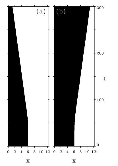
FIG. 1.: The NIB bifurcation in the 2:1 resonance: space-time plots showing an unstable stationary $\pi$-front (Ising) evolving into left (a) and right (b) traveling $\pi$-fronts (Bloch) beyond the NIB bifurcation.

In this paper we report on a new instability of $\pi$-fronts, occurring within the 4:1 band. Upon decreasing the forcing strength a stationary $\pi$-front loses stability and decomposes into a pair of traveling $\pi/2$ fronts. The instability is demonstrated in Fig. 2. The decomposition into a pair of traveling $\pi/2$-fronts is accompanied by the appearance of an intermediate (grey) domain whose phase of oscillation is shifted by $\pi/2$ with respect to the adjacent white and black domains. Like the NIB bifurcation the $\pi$-front instability within the 4:1 band designates a transition from stationary patterns to traveling waves. The significant difference is that the two-phase stationary patterns give place to traveling four-phase patterns. This feature of the 4:1 resonance is related to a peculiar property of the $\pi$-front instability to be discussed in Section III. The $\pi$-front decomposition instability appears to exist in higher $2n$:1 bands as well. We analyze in detail the 4:1 resonance case and bring numerical evidence for the existence of this type of instability in the 6:1 and 8:1 resonances. A brief account of some of the results to be reported here has appeared in Ref. [10].

FIG. 2.: The decomposition instability in the 4:1 resonance: Space-time plots (solutions of Eqn. (2) showing the decomposition of an unstable $\pi$-front into a pair of $\pi/2$-fronts traveling to the left (a) or to the right (b). The pairs of $\pi/2$-fronts enclose grey colored domains whose oscillation phases are shifted by $\pi/2$ with respect to the black and white domains. Parameters in Eqn. (2): $\mu=1.0$, $\nu=0.02$, $\gamma_{4}=0.3$.

We consider an extended system that is close to a Hopf bifurcation and externally forced with a frequency about four times larger than the Hopf frequency. The set of dynamical fields ${\bf u}$ describing the spatio-temporal state of the system (e.g. set of concentrations in the BZ reaction) can be written as ${\bf u}={\bf u_{0}}A\exp{(i\frac{\omega_{f}}{4}t)}+c.c.+\dots$, where ${\bf u_{0}}$ is constant, $A$ is a slowly varying complex amplitude, $\omega_{f}$ is the forcing frequency and the ellipses denote smaller contributions. The equation for the amplitude $A$ can be written in the following standard form (after rescaling and shifting $\arg{A}$ by a constant phase) [11, 12, 13, 14]:

$$A_{\tau} = (\mu+i\nu)A+(1+i\alpha)A_{zz}-(1-i\beta)|A|^{2}A$$ (2)

$$\mbox{}+\gamma_{4}{A^{\ast}}^{3}\,,$$

where the subscripts $\tau$ and $z$ denote partial derivatives with respect to time and space, and all the parameters are real. The proximity to the Hopf bifurcation implies $\mu<<1$. We will also be using the following form of Eqn. (2) obtained by rescaling time space and amplitude as $t=\mu\tau$, $x=\sqrt{\mu/2}z$ and $B=A/\sqrt{\mu}$:

$$B_{t} = (1+i\nu_{0})B+\frac{1}{2}(1+i\alpha)B_{xx}-(1-i\beta)|B|^{2}B$$ (4)

$$\mbox{}+\gamma_{4}{B^{\ast}}^{3}\,,$$

where $\nu_{0}=\nu/\mu$.

II Front solutions

We first study the gradient version of Eqn. (4) which is obtained by setting $\nu_{0}=\alpha=\beta=0$:

$$B_{t}=B+\frac{1}{2}B_{xx}-|B|^{2}B+\gamma_{4}{B^{*}}^{3}\,.$$ (5)

Eqn. (5) has four stable phase states for $0<\gamma_{4}<1$ shown by solid circles in Fig. 3: $B_{\pm 1}=\pm\lambda$ and $B_{\pm i}=\pm i\lambda$, where $\lambda=1/\sqrt{{1-\gamma_{4}}}$. Front solutions connecting pairs of these states divide into two groups, $\pi$-fronts and $\pi/2$-fronts. The $\pi$-fronts, shown in Fig. 3 as solid lines, are given by

$$B_{-1\to+1} = B_{+1}\tanh{x}\,,$$ (6)

$$B_{-i\to+i} = B_{+i}\tanh{x}\,.$$ (7)

The $\pi/2$-fronts are shown in Fig. 3 by the dashed curves. For the particular parameter value $\gamma_{4}=1/3$ they have the simple forms

$$B_{+1\to+i} = \frac{1}{2}\sqrt{\frac{3}{2}}\bigl{[}1+i-(1-i)\tanh{x}\bigr{]}\,,$$ (8)

$$B_{-i\to+1} = \frac{1}{2}\sqrt{\frac{3}{2}}\bigl{[}1-i+(1+i)\tanh{x}\bigr{]}\,,$$ (9)

$$B_{+i\to-1} = -B_{-i\to+1}\,,$$ (10)

$$B_{-1\to-i} = -B_{+1\to+i}\,.$$ (11)

Additional front solutions follow from the invariance of Eqn. (5) under reflection, $x\to-x$. For example, the symmetric counterparts of $B_{+i\to+1}(x)$ and $B_{+1\to-i}(x)$ are $B_{+1\to+i}(x)=B_{+i\to+1}(-x)$ and $B_{-i\to+1}(x)=B_{+1\to-i}(-x)$.

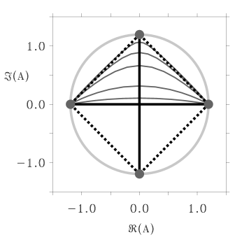
FIG. 3.: Phase portrait in the complex plane of solutions to Eqn. (5). The dots represent the 4 spatially uniform phase locked solutions. The solid lines are the $\pi$ front solutions and the dashed lines are the $\pi/2$ fronts. The thin lines in the circle are the phase portrait of showing the collapse of a $\pi$ front into two $\pi/2$ fronts.

Consider now the nongradient system (4). The main effect of the nongradient terms is to make the $\pi/2$-fronts traveling. The nongradient terms have no effect on the $\pi$-fronts which remain stationary. To see this we assume a traveling solution $B(x-ct)$ of Eqn. (4) and project this equation on the translational mode $B^{\prime}$. For $\pi$-fronts we obtain

$$c<{B_{0}^{\prime}}^{2}>=0\qquad B_{0}(z)=\lambda\tanh{z}\,,$$ (12)

implying $c=0$ (the brackets denote integration over the whole line). For $\pi/2$-fronts with $\gamma_{4}=1/3$ we find

$$|c| = \frac{\lambda}{<{B_{0}^{\prime}}^{2}>}\Bigl{[}(\nu_{0}+\frac{1}{2}\lambda^{2}\beta)<{B_{0}^{\prime}}>+\frac{1}{2}\beta<{B_{0}^{2}B_{0}^{\prime}}>\Bigr{]}$$ (13)

$$= \frac{3}{2}(\nu_{0}+\beta)\,,$$ (14)

where $\lambda=\sqrt{3/2}$. A perturbation analysis around $\gamma_{4}=1/3$ shows that the expression (14) for the speed remains valid for small deviations of $\gamma_{4}$ from $1/3$.

III A $\Pi$-front Instability

The $\pi$-fronts (6) are similar to the Ising front in the 2:1 band but as we will see shortly the instability they undergo is not a pitchfork bifurcation like the NIB. It is rather a degenerate instability leading to asymptotic solutions that are not smooth continuations of the unstable stationary $\pi$-fronts in a sense to be made clear in the following. A stability analysis of the $\pi$-fronts indicates that they lose stability at $\gamma_{4}=1/3$. To analyze the instability we study Eqn. (4) near that critical value.

A Gradient system

We begin with the gradient version (5). Introducing the new variables

$$U=\Re(B)+\Im(B)\qquad V=\Re(B)-\Im(B)\,,$$ (15)

we rewrite Eqn. (5) as

$$U_{t} = U+\frac{1}{2}U_{xx}-\frac{2}{3}U^{3}-\frac{d}{2}(U^{2}-3V^{2})U\,,$$ (17)

$$V_{t} = V+\frac{1}{2}V_{xx}-\frac{2}{3}V^{3}-\frac{d}{2}(V^{2}-3U^{2})V\,,$$ (18)

where

$\displaystyle d=\gamma_{4}-1/3\,.$

At the instability point, $\gamma_{4}=1/3$, the two equations decouple (since $d=0$) and admit solutions of the form

$$U = \sigma_{1}B_{0}(x-x_{1})\,,$$ (19)

$$V = \sigma_{2}B_{0}(x-x_{2})\,,$$ (20)

where $B_{0}(x)=\sqrt{\frac{3}{2}}\tanh{x}$, $\sigma_{1,2}=\pm 1$, and $x_{1}$ and $x_{2}$ are arbitrary constants. An intuitive understanding of this family of solutions can be obtained by expressing these solutions back in terms of the complex amplitude $B$. For $\sigma_{1}=-\sigma_{2}=1$ for example, the solution (19) is equivalent to

$\displaystyle B(x;x_{1},x_{2})=B_{-i\rightarrow+1}(x-x_{1})+B_{+1\rightarrow+i}(x-x_{2})-\lambda\,.$

When $|x_{2}-x_{1}|\rightarrow\infty$ this form approaches a pair of isolated $\pi/2$-fronts:

$\displaystyle B\approx B_{-i\rightarrow+1}(x-x_{1})\,,\qquad x\approx x_{1}\,,$

and

$\displaystyle B\approx B_{+1\rightarrow+i}(x-x_{2})\,,\qquad x\approx x_{2}\,.$

When $x_{2}-x_{1}=0$ it reduces to the $\pi$-front $B_{-i\rightarrow+i}$. Defining a “center of mass” coordinate, $\zeta$, and an order parameter, $\chi$, by

$\displaystyle\zeta=\frac{1}{2}(x_{1}+x_{2})\,,\qquad\chi=\frac{1}{2}(x_{2}-x_{1})\,,$

the one-parameter family of solutions, $\{\tilde{B}(x;\zeta,\chi)~{}|~{}\chi\in R\}$, where $\tilde{B}(x;\zeta,\chi)=B(x;x_{1},x_{2})$, represents $\pi/2$-front pairs with distances, $2\chi$, ranging from zero to infinity.

For $|\gamma_{4}-1/3|=|d|\ll 1$, the weak coupling between the two equations (17) and (18) induces slow drift along the solution family $B(x;x_{1},x_{2})$. We now write a pair solution as

$$U = \sigma_{1}B_{0}[x-x_{1}(t)]+u\,,$$ (21)

$$V = \sigma_{2}B_{0}[x-x_{2}(t)]+v\,,$$ (22)

where $u$ and $v$ are corrections of order $d$. Inserting these forms in Eqns. (15) we obtain

$${\cal H}_{1}u = \sigma_{1}\dot{x}_{1}B_{0}^{\prime}(x-x_{1})$$ (23)

$$- \frac{1}{2}d\sigma_{1}\bigl{[}B_{0}^{2}(x-x_{1})-3B_{0}^{2}(x-x_{2})\bigr{]}B_{0}(x-x_{1})\,,$$ (24)

$${\cal H}_{2}v = \sigma_{2}\dot{x}_{2}B_{0}^{\prime}(x-x_{2})$$ (25)

$$- \frac{1}{2}d\sigma_{2}\bigl{[}B_{0}^{2}(x-x_{2})-3B_{0}^{2}(x-x_{1})\bigr{]}B_{0}(x-x_{2})\,,$$ (26)

where ${\cal H}_{1,2}=-1-\frac{1}{2}\frac{\partial^{2}}{\partial x^{2}}+2B_{0}^{2}(x-x_{1,2})$. Projecting the right hand side of Eqn. (23) onto $B_{0}^{\prime}(x-x_{1})$, the zero eigenmode of ${\cal H}_{1}^{\dagger}={\cal H}_{1}$, and setting to zero we obtain

$$\dot{x}_{1} = -\frac{27}{16}d\int_{-\infty}^{\infty}dx$$ (28)

$$\mbox{}\times\tanh(x-x_{1})~{}{\rm sech}^{2}(x-x_{1})~{}\tanh^{2}(x-x_{2})\,,$$

A similar solvability condition for (25) leads to

$$\dot{x}_{2} = -\frac{27}{16}d\int_{-\infty}^{\infty}dx$$ (30)

$$\mbox{}\times\tanh(x-x_{2})~{}{\rm sech}^{2}(x-x_{2})~{}\tanh^{2}(x-x_{1})\,.$$

Expressing these equations in terms of $\zeta$ and $\chi$ we find

$$\dot{\zeta}=0\,,$$ (31)

$$\dot{\chi}=-\frac{27}{16}dJ(\chi)\,,$$ (32)

where

$$J(\chi)=\int_{-\infty}^{\infty}dz~{}\tanh{z}~{}{\rm sech}^{2}{z}~{}\tanh^{2}(z+2\chi)\,.$$ (33)

Evaluation of the integral in (33) yields

$$J(\chi) = I(a)=6(a^{-1}-a^{-3})+(1-3a^{-2})G(a)\,,$$ (34)

$$G(a) = (1-a^{-2})\ln\Bigr{(}\frac{1+a}{1-a}\Bigl{)}\,,$$ (35)

where $a=\tanh{2\chi}$. Note that Eqns. (31) and (32) are valid to all orders in $\chi$ and to linear order around $\gamma_{4}=1/3$.

The equation for the order parameter (32) can be written in the gradient form

$$\dot{\chi}=-\frac{dV}{d\chi}\,,\qquad V=\frac{27}{16}d\int^{\chi}J(z)dz\,.$$ (36)

Fig. 4 shows the potential $V(\chi)$ for $d>0$ ($\gamma_{4}>1/3$) and $d<0$. There is only one extremum point, $\chi=0$, of $V$. For $d>0$ it is a minimum and $\chi$ converges to zero. Pairs of $\pi/2$-fronts with arbitrary initial separation, $x_{2}-x_{1}$, attract one another and eventually collapse to a single $\pi$-front ($x_{1}=x_{2}$ or $\chi=0$). In practice, the collapse process is noticeable only for relatively small separations. For $d<0$ the extremum point, $\chi=0$, is a maximum and $\chi$ diverges to $\pm\infty$. A $\pi$-front decomposes into a pair of $\pi/2$-fronts which repel one another. This process is shown in Fig. 2 for the nongradient system (2). In the gradient case both $\pi$ and$\pi/2$-fronts are stationary (in the absence of interactions). Since the potential $V(\chi)$ becomes practically flat at finite $\chi$ values, the pair of $\pi/2$-fronts do not seem to depart from one another at long times. Fig. 3 shows the decomposition process of a $\pi$-front in the complex $B$ plane. Starting with the $B_{-1\to+1}$ $\pi$-front, represented by the thick solid phase portrait, the time evolution (thin solid phase portraits) is toward the fixed point $B_{+i}$ and the dashed phase portraits representing the pair of $\pi/2$-fronts $B_{+1\to+i}$ and $B_{+i\to-1}$. Because of the parity symmetry $\chi\to-\chi$, an appropriate perturbation of the initial $B_{-1\to+1}$ $\pi$-front could have led the dynamics toward the pair $B_{+1\to-i}$ and $B_{-i\to-1}$. Notice that for $d=0$, $\dot{\zeta}=0$, $\dot{\chi}=0$, and we recover the two-parameter family of pair solutions $B(x;\zeta,\chi)$ with arbitrary $\zeta$ and $\chi$. This degeneracy of solutions at $d=0$ is lifted by higher order terms in the amplitude equation (2) as will be discussed in Section III C below.

FIG. 4.: The potential $V(\chi)$. (a) For $d>0$ the extremum at $\chi=0$ is a minimum and and $\chi$ converges to $0$. (b) For $d<0$ the extremum is a maximum and $\chi$ diverges to $\pm\infty$.

B Nongradient system

The results described above can easily be extended to the nongradient system (4) for small $\alpha$, $\beta$ and $\nu_{0}$. The equations for $U$ and $V$ are

$$U_{t} = U+\frac{1}{2}U_{xx}-\frac{2}{3}U^{3}-\frac{d}{2}(U^{2}-3V^{2})U\,,$$ (38)

$$\mbox{}+\nu_{0}V+\frac{\alpha}{2}V_{xx}+\frac{\beta}{2}(U^{2}+V^{2})V\,,$$

$$V_{t} = V+\frac{1}{2}V_{xx}-\frac{2}{3}V^{3}-\frac{d}{2}(V^{2}-3U^{2})V\,,$$ (40)

$$\mbox{}-\nu_{0}U-\frac{\alpha}{2}U_{xx}-\frac{\beta}{2}(U^{2}+V^{2})U\,.$$

Assuming $d$, $\alpha$, $\beta$ and $\nu_{0}$ are of the same order of magnitude we write a solution in the form (22), insert in Eqs. (40) and obtain

$${\cal H}_{1}u = \sigma_{1}\dot{x}_{1}B_{0}^{\prime}(x-x_{1})$$ (41)

$$- \frac{1}{2}d\sigma_{1}\bigl{[}B_{0}^{2}(x-x_{1})-3B_{0}^{2}(x-x_{2})\bigr{]}B_{0}(x-x_{1})$$ (42)

$$+ \nu_{0}\sigma_{2}B_{0}(x-x_{2})+\frac{1}{2}\alpha\sigma_{2}B_{0}^{\prime\prime}(x-x_{2})$$ (43)

$$+ \frac{1}{2}\beta\sigma_{2}\bigl{[}B_{0}^{2}(x-x_{1})+B_{0}^{2}(x-x_{2})\bigr{]}B_{0}(x-x_{2})\,,$$ (44)

$${\cal H}_{2}v = \sigma_{2}\dot{x}_{2}B_{0}^{\prime}(x-x_{2})$$ (45)

$$- \frac{1}{2}d\sigma_{2}\bigl{[}B_{0}^{2}(x-x_{2})-3B_{0}^{2}(x-x_{1})\bigr{]}B_{0}(x-x_{2})$$ (46)

$$- \nu_{0}\sigma_{1}B_{0}(x-x_{1})-\frac{1}{2}\alpha\sigma_{1}B_{0}^{\prime\prime}(x-x_{1})$$ (47)

$$- \frac{1}{2}\beta\sigma_{1}\bigl{[}B_{0}^{2}(x-x_{1})+B_{0}^{2}(x-x_{2})\bigr{]}B_{0}(x-x_{1})\,.$$ (48)

Solvability conditions lead to equations for $\chi$ and $\zeta$. The equation for $\chi$ remains unchanged. That is, Eqn. (32) is valid for the nongradient equation (4) as well. The equation for $\zeta$ becomes

$$\sigma_{1}\sigma_{2}\dot{\zeta}=\nu_{0}F_{\nu}(\chi)+\alpha F_{\alpha}(\chi)+\beta F_{\beta}(\chi)\,,$$ (49)

where

$$F_{\nu} = -\frac{3}{4}G(a)-\frac{3}{2}a^{-1}\,,$$ (50)

$$F_{\alpha} = \frac{3}{4}I(a)\,,$$ (51)

$$F_{\beta} = 3a^{-1}\bigl{(}1-\frac{3}{2}a^{-2}\bigr{)}-\frac{9}{4}a^{-2}G(a)\,.$$ (52)

Notice that $F_{\nu}$, $F_{\alpha}$, and $F_{\beta}$ are odd functions of $\chi$ and do not vanish when $d=0$. When $|\chi|\to\infty$ the right hand side of (49) converges to $\frac{3}{2}(\nu_{0}+\beta)$, the speed of a $\pi/2$-front solution of Eqn. (4). The odd symmetries of $F_{\nu}$, $F_{\alpha}$, and $F_{\beta}$ imply that the $\chi=0$ solution (representing a $\pi$-front) remains stationary ($\dot{\zeta}=0$) in the nongradient case as well, and that the two pairs of $\pi/2$-fronts $\chi=\pm\infty$ propagate in opposite directions.

C The effect of higher order terms

According to Eqn. (32) the asymptotic solutions just below $\gamma_{4}=1/3$, the $\pi/2$-front pairs as $|\chi|\to\infty$, are not smooth continuations of the stationary $\pi$-front at $\gamma_{4}=1/3$ (the $\chi=0$ solution). This abrupt nature of the instability is related to a degeneracy of solutions at $\gamma_{4}=1/3$. At this parameter value a whole family of solutions exists describing $\pi/2$-front pairs with distances $|x_{2}-x_{1}|=2|\chi|$ ranging from zero to infinity. In the nongradient case these pair solutions propagate at speeds given by Eqn. (49). The degeneracy of solutions is lifted by higher order terms in Eqn. (4).

Consider the gradient version of the amplitude equation

$$B_{t}=B+\frac{1}{2}B_{xx}-|B|^{2}B+\gamma_{4}{B^{*}}^{3}+\mu H(B,B^{*};\partial_{x})\,,$$ (53)

where $H(B,B^{*};\partial_{x})$ includes higher order terms like $|B|^{4}B$, $|B|^{2}B_{xx}$, etc.. The factor $\mu$ reflects the fact that fifth order terms in the amplitude equation are smaller by factor $\mu\ll 1$ than the lower order terms. The effect of these terms is generally weak, but becomes important near $\gamma_{4}=1/3$. Consider, for example, the effect of the term $\delta|B|^{2}B_{xx}$. Eqs. (15) include now the contributions

$\displaystyle\frac{1}{2}\mu\delta(U^{2}+V^{2})U_{xx}\quad{\rm and}\quad\frac{1}{2}\mu\delta(U^{2}+V^{2})V_{xx}\,,$

respectively. The corresponding contributions to Eqs. (23) and (25) are

$\displaystyle\frac{1}{2}\mu\delta\sigma_{1}\bigl{[}B_{0}^{2}(x-x_{1})+B_{0}^{2}(x-x_{2})\bigr{]}B_{0}^{\prime\prime}(x-x_{1})$

and

$\displaystyle\frac{1}{2}\mu\delta\sigma_{2}\bigl{[}B_{0}^{2}(x-x_{1})+B_{0}^{2}(x-x_{2})\bigr{]}B_{0}^{\prime\prime}(x-x_{2})\,.$

The equation for the order parameter will now read

$$\dot{\chi}=-\frac{27}{16}dJ(\chi)+\frac{9}{8}\delta\mu K(\chi)\,,$$ (54)

where

$$K(\chi)=\int_{-\infty}^{\infty}dz~{}\tanh{z}~{}{\rm sech}^{4}{z}~{}\tanh^{2}(z+2\chi)\,.$$ (55)

The integral (55) is elementary but the expression is lengthy and we do not display it here. The second term on the right hand side of Eqn. (54), whose origin is the fifth order term $|B|^{2}B_{xx}$, cannot be neglected in a $\mu$-neighborhood of $\gamma_{4}=1/3$. Depending on the sign of $\delta$ two scenarios are possible as $\gamma_{4}$ is decreased. In both cases the $\chi=0$ ($\pi$-front) solution is destabilized at $\gamma_{4c}=1/3+8\mu\delta/21$. When $\delta>0$ the $\chi=0$ solution is destabilized to a new pair of solutions, $\chi_{\pm}$, in a pitchfork bifurcation. For $|\chi|\ll 1$ the new solutions assume the approximate values, $\chi_{\pm}\approx\pm\frac{\sqrt{21}}{4}\sqrt{1-d/d_{c}}$, where $d_{c}=\gamma_{4c}-1/3$. When $\gamma_{4}$ is further decreased the two stable solutions $\chi_{\pm}$ move to $\pm\infty$ on a $\gamma_{4}$ range of order $\mu$. When $\delta<0$ bistability of the $\chi=0$ solution and the $\chi=\pm\infty$ solutions first develop. As $\gamma_{4}$ is further decreased the $\chi=0$ solution becomes metastable until it loses completely its stability at $\gamma_{4c}$. Fig. 5 shows the potential

$$V=\frac{9}{8}\int^{\chi}\Bigl{[}\frac{3}{2}dJ(z)-\delta\mu K(z)\Bigr{]}dz\,,$$ (56)

associated with Eqn. (54) for both scenarios.

FIG. 5.: The effects of the higher order term $\delta|B|^{2}B_{xx}$ on the decomposition instability within the 4:1 resonance. The potential (56) deforms from a single well to a single barrier as $\gamma_{4}$ is decreased past $\gamma_{4c}$. In the intermediate range two scenarios are possible: (a) For $\delta>0$, the $\chi=0$ solution loses stability in a pitchfork bifurcation at $\gamma_{4c}$ to a pair of solutions that move to $\pm\infty$. Parameters: $\delta=1.0$, $\mu=0.01$, $\gamma_{4}=0.339,0.337,0.336,0.335,0.333$. (b) For $\delta<0$, the $\chi=0$ solution remains stable while the $\chi=\pm\infty$ solutions acquire stability and loses stability only below $\gamma_{4c}$. Parameters: $|\delta|=1.0$, $\mu=0.01$, $\gamma_{4}=0.334,0.332,0.331,0.330,0.328$. In both scenarios the deformations from a single well to a single barrier occur within a small range of $\gamma_{4}$ of order $\mu\ll 1$. For comparison, an equivalent figure for the degenerate case ($\delta=0$) is shown in (c). The only intermediate form between a single well and a single barrier is a flat potential, $V=0$, ocurring at $\gamma=1/3$.

The two scenarios are related by the symmetry $d\to-d$, $\delta\to-\delta$, $t\to-t$ of Eqn. (54). The first scenario ($\delta>0$) amounts to a pitchfork bifurcation from a stable $\chi=0$ solution to a pair of stable $\chi_{\pm}$ solutions that move to infinity as $\gamma_{4}$ is decreased. The second scenario ($\delta<0$) amounts to a backward pitchfork bifurcation from an unstable $\chi=0$ solution to a pair of unstable $\chi_{\pm}$ solutions that move to infinity as $\gamma_{4}$ is increased.

The higher order term $|B|^{2}B_{xx}$, and similarly other high order terms, lift the degeneracy of the lower order system (5) at $\gamma_{4}=1/3$. For $\delta>0$ and in a small $\gamma_{4}$ range of order $\mu$ near 1/3 the instability becomes similar to the NIB bifurcation in the 2:1 resonance. But apart from the behavior in this small parameter range the overall behavior does not change: a $\pi$-front decomposes into a pair of $\pi/2$-fronts as $\gamma_{4}$ is decreased.

IV $\Pi$-front instabilities in higher resonances

We have found numerical evidence for the existence of similar $\pi$-front instabilities within the 6:1 and 8:1 bands. These findings suggest the following generalization: within the $2n$:1 band ($n>1$) a $\pi$-front may lose stability by decomposing into $n$ $\pi/n$-fronts. Consider the equation

$$B_{t} = \frac{1}{2}B_{xx}+(1+i\nu_{0})B$$ (59)

$$\mbox{}+\mu_{4}|B|^{2}B+\mu_{6}|B|^{4}B+\mu_{8}|B|^{6}B$$

$$\mbox{}+\gamma_{4}{B^{*}}^{3}+\gamma_{6}{B^{*}}^{5}+\gamma_{8}{B^{*}}^{7}\,.$$

The normal form equation up to seventh order contains many more terms. Our purpose here, however, is just to demonstrate the $\pi$-front instability for some parameter values pertaining to the 6:1 and 8:1 bands. Fig. 6 shows the decomposition in the complex $B$ plane of a $\pi$-front within the 6:1 band into three $\pi/3$-fronts. Fig. 7 shows the decomposition of a $\pi$-front within the 8:1 band into four $\pi/4$-fronts.

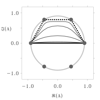
FIG. 6.: Decomposition if a $\pi$ front into three $\pi/3$ fronts in the 6:1 resonance band. Parameters in Eqn. (59): $\gamma_{6}=0.9$, $\mu_{4}=-1.0$, $\mu_{6}=-1.0$. All other parameters are zero.

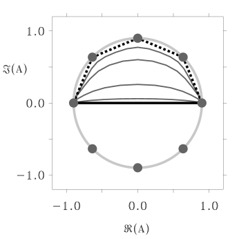
FIG. 7.: Decomposition if a $\pi$ front into four $\pi/4$ fronts in the 8:1 resonance band. Parameters in Eqn. (59): $\gamma_{8}=0.75$, $\mu_{4}=-0.5$, $\mu_{6}=-0.5$, $\mu_{8}=-1.0$. All other parameters are zero.

Fig. 8 shows a space-time plot of the decomposition instability within the 6:1 band. The initial unstable $\pi$-front decomposes into three $\pi/3$-fronts, traveling to the left or to the right depending on initial conditions. Along with this process two intermediate phase states appear between the original white and black phases.

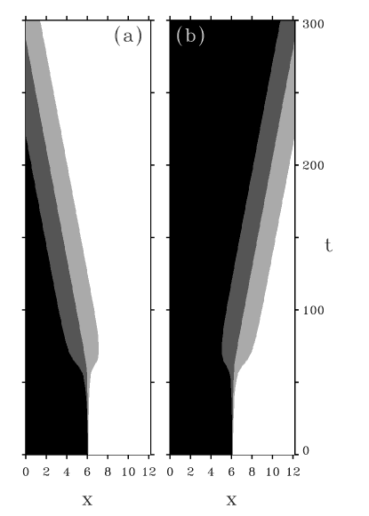
FIG. 8.: Decomposition if a $\pi$ front into three $\pi/3$ fronts in the 6:1 resonance band. The figures show space-time plots of numerical solutions of Eqn. (59) with parameters $\gamma_{6}=0.9$, $\mu_{4}=-1.0$, $\mu_{6}=-1.0$, $\nu_{0}=0.1$. All other parameters are zero.

V Implications on pattern formation

The $\pi$-front instability in the 4:1 band has a pronounced effect on patterns. Despite the coexistence of four uniform phase states and the stability of $\pi/2$-fronts, asymptotic four-phase patterns appear only below the $\pi$-front instability point $\gamma_{4}=1/3$. The reason is the attractive interactions between $\pi/2$-fronts when $\gamma_{4}>1/3$ and the collapse into $\pi$-fronts. Thus, for $\gamma_{4}>1/3$ two-phase patterns prevail. These patterns form standing waves since $\pi$-fronts are stationary. For $\gamma_{4}<1/3$ the interaction between $\pi/2$-fronts is repulsive and four-phase patterns prevail. These patterns travel since $\pi/2$-fronts propagate.

Fig. 9$a$ shows a stably rotating four-phase spiral wave for $\gamma_{4}<1/3$. Figs. 9$b,c,d$ show the collapse of this spiral wave into a stationary two-phase pattern as $\gamma_{4}$ is increased past $1/3$. The collapse begins at the spiral core where the $\pi/2$-front interactions are the strongest. As pairs of $\pi/2$-fronts attract and collapse into $\pi$-fronts, the core splits into two vertices that propagate away from each other leaving behind a two-phase pattern.

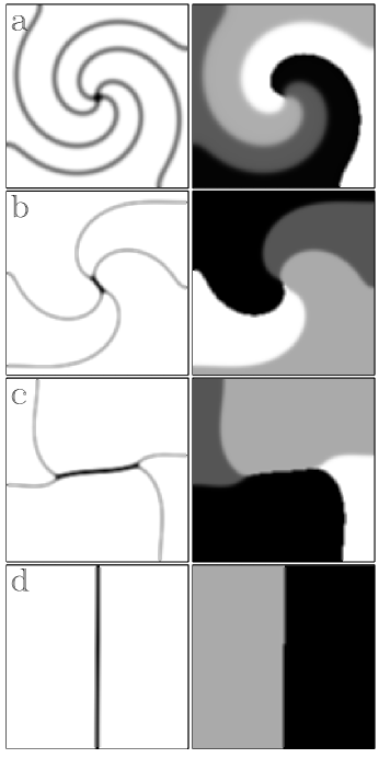
FIG. 9.: Numerical solution of a two-dimensional version of Eqn. (4) showing the collapse of a rotating four-phase spiral-wave into a stationary two-phase pattern. The left column is $|A|$ and the right column $\arg(A)$ in the $x-y$ plane. (a) The initial four-phase spiral wave (computed with $\gamma_{4}<1/3$). (b) The spiral core, a 4-point vertex, splits into two 3-point vertices connected by a $\pi$-front. (c) A two-phase pattern develops as the 3-point vertices further separate. (d) The final stationary two-phase pattern. Parameters: $\gamma_{4}=0.6$, $\nu_{0}=0.1$, $\alpha=\beta=0$, $x=[0,64]$, $y=[0,64]$.

REFERENCES

• [1] D. Walgraef, ”Spatio-Temporal Pattern Formation” (Springer-Verlag, New York, 1997).
• [2] P. Coullet and K. Emilsson, Physica D 61, 119 (1992).
• [3] B. A. Malomed and A. A. Nepomnyashcy, Europhys. Lett. 27, 649 (1994).
• [4] P. Coullet, J. Lega, B. Houchmanzadeh, and J. Lajzerowicz, Phys. Rev. Lett. 65, 1352 (1990).
• [5] A. Hagberg and E. Meron, Nonlinearity 7, 805 (1994).
• [6] M. Bode, A. Reuter, R. Schmeling, and H.-G. Purwins, Phys Lett. A 185, 70 (1994).
• [7] C. Elphick, A. Hagberg, E. Meron, and B. Malomed, Phys. Lett. A 230, 33 (1997).
• [8] V. Petrov, Q. Ouyang, and H. L. Swinney, Nature 388, 655 (1997).
• [9] B. Krauskopf, Ph.D. thesis, Rijksuniversiteit Groningen, 1995.
• [10] C. Elphick, A. Hagberg, and E. Meron, Phys. Rev. Lett. 80, 5007 (1998).
• [11] A. C. Newell, Lect. App. Math. 15, 157 (1974).
• [12] J. M. Gambaudo, J. Diff. Eq. 57, 172 (1985).
• [13] C. Elphick, G. Iooss, and E. Tirapegui, Phys. Lett. A 120, 459 (1987).
• [14] M. C. Cross and P. C. Hohenberg, Rev. of Mod. Phys. 65, 851 (1993).