Two-color nonlinear localized photonic modes

Abstract

We analyze second-harmonic generation (SHG) at a thin effectively quadratic nonlinear interface between two linear optical media. We predict multistability of SHG for both plane and localized waves, and also describe two-color localized photonic modes composed of a fundamental wave and its second harmonic coupled together by parametric interaction at the interface.

Cascaded nonlinearities of noncentrosymmetric optical materials have become an active topic of research over the last years due to their potential applications in all-optical switching devices [1]. Parametric interaction is known also to support solitary waves, in particular spatial quadratic solitons, which are two-frequency self-trapped beams consisting of a fundamental wave parametrically coupled to its second-harmonic [2]. Usually, solitary waves are considered for homogeneous media where spatial localization is induced by self-focusing and self-trapping effects. However, localized modes can exist even in a linear medium at defects or interfaces, and they are known as linear defect or interface modes. The properties of nonlinear defect modes are usually analyzed for nonresonant Kerr-type nonlinearities [3]. Here we consider a qualitatively different situation and introduce another type of nonlinear defect mode: a two-frequency (or two-color) localized photonic mode, where the energy is localized due to the parametric wave mixing induced by an interface between two linear optical media or a thin layer with a quadratic (or $\chi^{(2)}$) nonlinearity embedded in a linear bulk medium.

The physical motivation for our model is twofold. First of all we point out a fundamental property of inhomogeneous nonlinear optical media. Let us consider an interface between two semi-infinite bulk optical media, which are either clamped together or separated by an infinitely thin layer. If the bulk medium has inversion symmetry, then its quadratic nonlinearity must vanish. However, the interface breaks the symmetry and therefore the interface nonlinearity should possess a nonvanishing quadratic response, due to a nonzero contribution from the spatial derivatives of the electric field [4].

Second, there exists a strong experimental evidence of SHG in localized photonic modes. For example, recent experimental results [5] reported SHG in a truncated one-dimensional periodic photonic band-gap structure, in which a nonlinear defect layer was embedded. An enhancement of the parametric interaction in the vicinity of the defect was observed, suggesting that SHG occurs in local modes, while being completely suppressed for other propagating modes. If the band gap of the periodic structure is wide, we can describe this SHG process by a model with a local quadratic nonlinear defect.

The main purpose of this paper is to introduce and study an analytically solvable model for SHG in nonlinear localized modes, based on the (induced or inherent) quadratic nonlinearity of an interface separating two (generally different) linear bulk media or a thin nonlinear defect layer embedded in a bulk medium. In particular, we describe two-color localized nonlinear defect modes where the energy localization occurs due to parametric coupling at the interface.

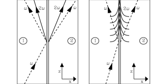
FIG. 1.: Scattering of a plane FF wave (dashed) on a $\chi^{(2)}$-interface between two linear media 1 and 2. The generated SH (solid) can be either propagating or localized.

We consider a fundamental frequency (FF) wave propagating along the $Z$ direction in a linear slab waveguide, as shown in Fig. 1. We assume that an interface (or defect layer) at $x$=0 possesses a quadratic nonlinear response, so that the FF wave can parametrically couple to its second harmonic (SH) at the interface [4]. The coupled-mode equations for the complex envelope functions $E_{j}(x,Z)$ ($j$=1,2) can then be written in the form

$$\begin{array}[]{l}{\displaystyle i\frac{\partial E_{1}}{\partial Z}+D_{1}\frac{\partial^{2}E_{1}}{\partial x^{2}}+n_{1}(x)E_{1}+\Gamma_{1}(x)E_{1}^{*}E_{2}=0,}\\[9.0pt] {\displaystyle i\frac{\partial E_{2}}{\partial Z}+D_{2}\frac{\partial^{2}E_{2}}{\partial x^{2}}+n_{2}(x)E_{2}+\Gamma_{2}(x)E_{1}^{2}=0,}\end{array}$$ (1)

where $D_{j}$ are diffraction coefficients ($D_{j}>0$). For the geometry shown in Fig. 1 and the approximation of an infinitely thin interface layer (valid when the width of the layer is much smaller than the FF wavelength), we take $n_{j}(x)=n_{0j}(x)+\kappa_{j}\delta(x)$ and $\Gamma_{j}(x)=\gamma_{j}\delta(x)$, where $\gamma_{j}$ are the nonlinearity coefficients, $\kappa_{j}$ account for the phase velocity differences in the layer and bulk materials, and $n_{0j}(x)=n_{0j}^{+}$, for $x>0$, and $n_{0j}(x)=n_{0j}^{-}$, for $x<0$.

In order to reduce the number of parameters we normalize Eqs. (1) as follows: $E_{1}(Z)=u(z)/\sqrt{\gamma_{1}\gamma_{2}}$, $E_{2}(Z)=v(z)/\gamma_{1}$, $\sigma=D_{2}/D_{1}$, $\alpha_{1}=\kappa_{1}/D_{1}$, and $\alpha_{2}=\kappa_{2}/D_{1}$, where $z=Z/D_{1}$ is measured in units of $D_{1}$. Then the coupled equations take the form

$$\begin{array}[]{l}{\displaystyle i\frac{\partial u}{\partial z}+\frac{\partial^{2}u}{\partial x^{2}}+\nu_{1}\left(x\right)u+\delta\left(x\right)\left(\alpha_{1}u+u^{*}v\right)=0,}\\[9.0pt] {\displaystyle i\frac{\partial v}{\partial z}+\sigma\frac{\partial^{2}v}{\partial x^{2}}+\nu_{2}\left(x\right)v+\delta\left(x\right)\left(\alpha_{2}v+u^{2}\right)=0,}\end{array}$$ (2)

where $\nu_{j}(x)=\nu_{j}^{+}=n_{0j}^{+}/D_{1}$, for $x>0$, and $\nu_{j}(x)=\nu_{j}^{-}=n_{0j}^{-}/D_{1}$, for $x<0$. If the mismatch $2n_{01}^{\pm}-n_{02}^{\pm}$ is small then $\sigma$=1/2 is a good approximation, which we use below in the numerics. The system (2) conserves the Hamiltonian

$$H = \int_{-\infty}^{+\infty}{\left\{{\left|\frac{\partial u}{\partial x}\right|}^{2}+\frac{\sigma}{2}{\left|\frac{\partial v}{\partial x}\right|}^{2}-\nu_{1}(x){\left|u\right|}^{2}-\frac{\nu_{2}(x)}{2}{\left|v\right|}^{2}\right.}$$

$${\left.-\delta(x){\left[\alpha_{1}{\left|u\right|}^{2}+\frac{\alpha_{2}}{2}{\left|v\right|}^{2}+\textrm{Re}{\left(u^{2}v^{*}\right)}\right]}\right\}dx},$$

and the total power $P=\int_{-\infty}^{+\infty}\left(|u|^{2}+|v|^{2}\right)dx$ for spatially localized or periodic solutions.

Scattering problem. To analyze the scattering process we use that Eqs. (2) are linear for $x\neq 0$, and write the total field as a superposition of plane waves,

$$u(x,z) = \left\{\begin{array}[]{lr}a_{1}e^{-i\lambda_{1}z+i{q}_{1}^{-}x}+b_{1}e^{-i\lambda_{1}z-i{q}_{1}^{-}x};&x<0\\ c_{1}e^{-i\lambda_{1}z+i{q}_{1}^{+}x};&x>0,\end{array}\right.$$ (5)

$$v(x,z) = \left\{\begin{array}[]{lr}b_{2}e^{-i\lambda_{2}z-i{q}_{2}^{-}x};&x<0\\ c_{2}e^{-i\lambda_{2}z+i{q}_{2}^{+}x};&x>0,\end{array}\right.$$ (8)

where $a_{1}$, $b_{1}$, and $c_{1}$ are the amplitudes of the incident, reflected, and transmitted FF waves, respectively. Correspondingly, $b_{2}$ and $c_{2}$ are the amplitudes of the generated SH waves on both sides of the interface. The dispersion relations are then given by

$$\lambda_{1}={\left({q}_{1}^{\pm}\right)}^{2}-\nu_{1}^{\pm},\;\;\lambda_{2}=\sigma{\left({q}_{2}^{\pm}\right)}^{2}-\nu_{2}^{\pm},$$ (9)

and the continuity condition at $x$=0 yields the relations $a_{1}+b_{1}=c_{1}$ and $b_{2}=c_{2}$. Next, integrating Eqs. (2) over an infinitely small segment around the interface, we obtain the relations between the field derivatives on opposite sides of the layer,

$${\displaystyle\begin{array}[]{rll}-{\left[\partial u/\partial x\right]}_{-0}^{+0}&=&{\left(u^{*}v+\alpha_{1}u\right)}|_{x=0},\\[9.0pt] -\sigma{\left[\partial v/\partial x\right]}_{-0}^{+0}&=&{\left(u^{2}+\alpha_{2}v\right)}|_{x=0}.\end{array}}$$ (10)

This gives the phase-matching condition $2\lambda_{1}=\lambda_{2}$, which is a general requirement for stationary propagation of FF and SH without energy exchange, and two algebraic relations for the amplitudes,

$$\begin{array}[]{l}{\displaystyle-i\left(q_{1}^{-}+q_{1}^{+}\right)c_{1}+2iq_{1}^{-}a_{1}=c_{1}^{*}c_{2}+\alpha_{1}c_{1},}\\[9.0pt] {\displaystyle-i\sigma\left(q_{2}^{-}+q_{2}^{+}\right)c_{2}=c_{1}^{2}+\alpha_{2}c_{2}.}\end{array}$$ (11)

All unknown parameters $q_{1}^{+}$, $q_{2}^{\pm}$, $\lambda_{j}$, $b_{j}$, and $c_{j}$ can now be expressed in terms of the amplitude $a_{1}$ and transverse wave number $q_{1}^{-}$ of the incident FF wave.

The SH amplitude at the interface is determined from Eq. (11),

$$c_{2}=-c_{1}^{2}/\left[\alpha_{2}+i\sigma\left(q_{2}^{-}+q_{2}^{+}\right)\right].$$ (12)

The wave numbers are found from the phase-matching condition $2\lambda_{1}=\lambda_{2}$ and the dispersion relations (9),

$$\begin{array}[]{l}{\displaystyle q_{1}^{+}=\sqrt{(q_{1}^{-})^{2}+\nu_{1}^{+}-\nu_{1}^{-}},}\\[9.0pt] {\displaystyle q_{2}^{\pm}=\sqrt{\left[2(q_{1}^{-})^{2}+\nu_{2}^{\pm}-2\nu_{1}^{-}\right]/\sigma}.}\end{array}$$ (13)

These values can be either real or imaginary, corresponding to plane waves and waves that are spatially localized at the interface, respectively. Note that the sign of the wave numbers is fixed according to the predefined geometry of the problem (see Fig. 1).

Multistability. Substituting Eq. (12) into Eq. (11) we obtain the characteristic equation for the FF wave intensity $|c_{1}|^{2}$ at the interface,

$$|c_{1}^{6}|-2|c_{1}^{4}|{\rm Re}(\widetilde{\alpha}_{1}\widetilde{\alpha}_{2})+|c_{1}^{2}|\left|\widetilde{\alpha}_{1}\widetilde{\alpha}_{2}\right|^{2}=4|a_{1}|^{2}|q_{1}^{-}\widetilde{\alpha}_{2}|^{2},$$ (14)

where $\widetilde{\alpha}_{1}=\alpha_{1}+i\left(q_{1}^{-}+q_{1}^{+}\right)$ and $\widetilde{\alpha}_{2}=\alpha_{2}+i\sigma\left(q_{2}^{-}+q_{2}^{+}\right)$. Equation (14) is cubic in $|c_{1}|^{2}$, and thus three different roots may exist for a given input intensity $|a_{1}|^{2}$, corresponding to three different values of the amplitudes at the interface, as shown in Fig. 2(a). This describes a multistable SHG process.

To study the stability of these solutions we investigate the corresponding linearized problem, similar to the analysis of a different problem in Ref. [6]. It is convenient to chose the perturbation functions with profiles which remain self-similar upon propagation in the inhomogeneous medium. Then it can be demonstrated that the growth rate for nonoscillatory instability modes vanishes at the turning points $\partial|a_{1}|^{2}/\partial|c_{1}|^{2}=0$. We have verified numerically that the growth rate is positive on the branch with negative slope [dashed line, Fig. 2(a)], meaning that the corresponding solutions are unstable. However, a rigorous stability analysis of all nonlinear modes is beyond the scope of this paper.

Let us consider the simplest possible example, in order to illustrate the characteristic physical properties of the system. We choose the case when the linear media 1 and 2 on each side of the interface (see Fig. 1) are identical, i.e., $\nu_{j}^{\pm}=\nu_{j}$. It then immediately follows from Eqs. (13) that $q_{j}^{\pm}=q_{j}$. This means that the SH can exist in two different states, propagating or localized, whereas the FF waves are always propagating. The localized SH state can only be observed if $\beta>0$, and then only for FF wave numbers less than a critical value: $q_{1}<\sqrt{\beta/2}$, where $\beta\equiv 2\nu_{1}-\nu_{2}$. Note that localization does not depend on the wave amplitudes.

For fixed material parameters $\alpha_{j}$ and $\beta$ the multistable SHG regime can only be observed in certain regions of the input parameters $q_{1}$ and $|a_{1}|^{2}$, as illustrated in Fig. 2(b). Importantly, multistability can be found for both propagating (region I) and localized (region II) SH waves. For other values of the material parameters the multistable scattering might be observed for a single type of the SH waves, or only a single-state field configuration may be possible.

FIG. 2.: (a) Dependence of incident FF intensity $|a_{1}|^{2}$ on FF intensity at the layer $|c_{1}|^{2}$, illustrating existence of multistability. (b) Regions of multistability in $(q_{1},|a_{1}|^{2})$–space for $\alpha_{1}$=1, $\alpha_{2}$=0.15, and $\beta$=0.02. The three SH solutions are propagating (region I) or localized (region II). Only one solution exists outside regions I and II. The dashed line $q_{1}$=0.09 corresponds to the case shown in (a).

In Fig. 3 we summarize the different SHG regimes in terms of the material parameters. The diagrams are presented for $\alpha_{1}=\pm 1$, but they are invariant to the scaling $\beta\rightarrow\beta/\alpha_{1}^{2}$, $\alpha_{2}\rightarrow\alpha_{2}/|\alpha_{1}|$, meaning that they can characterize the multistability regions for any $\alpha_{1}$.

FIG. 3.: Regions I-III in ($\beta,\alpha_{2}$)–space for $\alpha_{1}=\pm$1 where multistability can be observed. In region I all three SH states are propagating, in II they can be either propagating or localized, and in III they are all localized. The marked point corresponds to the case presented in Fig. 2.

Nonlinear localized modes. As mentioned above, in the scattering of a plane FF wave the transmitted FF and generated SH waves can be either propagating or localized. However, the situation when all the FF and SH waves are localized is also possible. These two-frequency nonlinear localized modes are of significant physical interest. To find stationary solutions for these modes we assume the following conditions in the general scattering problem: (i) no incident plane wave, i.e., $a_{1}$=0, and (ii) all transverse wave numbers are imaginary, $q_{j}^{\pm}=i\mu_{j}^{\pm}$, where $\mu_{j}^{\pm}$ are real and positive (as the wave amplitudes should vanish at infinity). Then the amplitudes at the interface are $|c_{1}|^{2}=\left(\mu_{1}^{-}+\mu_{1}^{+}-\alpha_{1}\right)\left[\sigma\left(\mu_{2}^{-}+\mu_{2}^{+}\right)-\alpha_{2}\right]$ and $c_{2}=\mu_{1}^{-}+\mu_{1}^{+}-\alpha_{1}$. Note that here only one wave number is arbitrary, all others are determined by Eq. (13). Such localized states can exist for any combination of material parameters. Some examples are presented in Figs. 4(a) and 4(b).

For the symmetric case, where $\nu_{j}^{\pm}=\nu_{j}$ and $\mu_{j}^{\pm}=\mu_{j}$, the total power $P=|c_{1}|^{2}/\mu_{1}+|c_{2}|^{2}/\mu_{2}$ can be written as a function of $\mu_{1}$ only. The dependence $P(\mu_{1})$ has always, for any values of the material parameters, a branch with positive slope. Under certain conditions a second branch with negative slope may appear. This branch corresponds to smaller values of $\mu_{1}$ and larger values of the Hamiltonian $H$, as shown in Figs. 4(c) and 4(d) with dashed lines. Thus we may conclude that for two bistable states the one with lower $\mu_{1}$ (i.e., higher $H$ and negative slope ${\partial P/\partial\mu_{1}}<0$) is unstable. For other values of the material parameters the power ranges corresponding to branches with positive and negative slope may not fully overlap, or there can even be a gap.

FIG. 4.: (a,b) Intensity profiles of two different localized states with the same power $P$=20 (FF – dashed, SH – solid). (c) Power $P(\mu_{1})$ with two branches. (d) Hamiltonian $H$ vs. power $P$. The unstable branch is depicted with a dashed line. Points a and b mark the modes shown in (a) and (b), respectively. For all the plots $\alpha_{1}=\alpha_{2}=-$1, $\beta=2$.

Let us consider the generation of a stable two-color localized mode by launching a localized FF wave at the interface. As the first step in the analysis of the dynamical problem we consider a simplified case, assuming that both the amplitude and phase velocity of the FF pump wave at the interface are constant. This is a reasonable approximation, if the initial FF wave is close to a stationary mode localized due to a linear phase detuning at the layer (characterized by $\alpha_{1}$), and the generated SH wave remains small (essentially an undepleted pump approximation). For such a case, the original system (2) can be reduced to a single equation for the SH wave,

$$i\frac{\partial v}{\partial z}+\sigma\frac{\partial^{2}v}{\partial x^{2}}+\nu_{2}v+\delta(x)\left(\alpha_{2}v+{\left|c_{10}^{2}\right|}e^{-2i\lambda_{1}z}\right)=0,$$ (15)

with the initial condition $v(0)$=0. In Eq. (15) the initial intensity of the FF wave at the interface $|c_{10}^{2}|$ and its propagation constant $\lambda_{1}$ are fixed.

In the case $\alpha_{2}$=0, an exact solution of Eq. (15) can be presented in the form,

$\displaystyle v(x,z)=e^{-2i\lambda_{1}z}\int_{0}^{z}{\frac{i{\left|c_{10}^{2}\right|}}{2\sqrt{i\pi\sigma\zeta}}e^{i\left(2\lambda_{1}+\nu_{2}\right)\zeta}e^{{ix^{2}}/{4\sigma\zeta}}d\zeta}.$

The expression under the integral describes decaying oscillations with the increase of $z$. Thus, the amplitude of the generated SH exhibits oscillations as the solution approaches asymptotically a stationary two-color localized state. We have performed a number of numerical simulations (using a fully implicit finite-difference method) with Gaussian initial profiles of the FF wave and found that in the general case the formation of localized modes is accompanied by the same kind of transitional oscillations, as shown in Fig. 5. Furthermore, we also observed switching from a perturbed unstable two-color localized mode, such as that shown in Fig. 4(a), to a stable one. In the evolution process some energy is radiated, and the power corresponding to the localized mode is decreased accordingly. Thus, a stable localized mode can only be generated, if initial power is above the threshold $P_{\rm th}={\rm min}_{\mu_{1}}P(\mu_{1})$.

FIG. 5.: Generation of a two-color localized mode (material parameters are the same as in Fig. 4). Left: intensities of the FF (dashed) and SH (solid) modes at the interface. Right: evolution of the excited SH. The input power is $P\simeq 28$ and the final state is close to that shown in Fig. 4(b).

In conclusion, we have introduced an analytically solvable model for SHG in localized modes and predicted the existence of two-color nonlinear localized photonic modes supported by parametric interaction at an interface. Some of the properties of two-color localized modes, such as stability, generation, and switching, show a remarkable similarity with parametric solitons in homogeneous optical $\chi^{(2)}$ media [2] and their interaction with localized perturbations of the mismatch parameter [7]. We believe that these results open a new class of problems in the theory of nonlinear wave propagation in inhomogeneous media with resonant nonlinearities, and they should be useful to understanding the fundamental difference between the effects produced by nonresonant Kerr-type nonlinearities and those induced by parametric wave interaction. For example, the analysis of localized modes due to a single $\chi^{(2)}$ defect is the first step towards the theory of nonlinear modes and gap solitons in nonlinear photonic crystals [8] and the dynamics of the defect modes in such materials.

The authors are indebted to C. Soukoulis and R. Vilaseca for useful discussions and comments. The work was partially supported by the Department of Industry, Science, and Tourism (Australia).

REFERENCES

- [1] For an overview, see G. Stegeman, D.J. Hagan, and L. Torner, Opt. Quantum Electron. 28, 1691 (1996).
- [2] Yu.N. Karamzin and A.P. Sukhorukov, Zh. Eksp. Teor. Fiz. 68, 834 (1975) [Sov. Phys. JETP 41, 414 (1976)]; A.V. Buryak and Yu.S. Kivshar, Phys. Lett. A 197, 407 (1995); D.E. Pelinovsky, A.V. Buryak, and Yu.S. Kivshar, Phys. Rev. Lett. 75, 591 (1995); L. Torner, In : Beam Shaping and Control with Nonlinear Optics, F. Kajzar and R. Reinisch, Eds. (Plenum, New York, 1998), p. 229.
- [3] For a general overview, see O.M. Braun and Yu.S. Kivshar, Phys. Rep. 306, 1 (1998), and references therein.
- [4] V.M. Agranovich and S.A. Darmanyan, JETP Lett. 35, 80 (1982) [Pis’ma Zh. Eksp. Teor. Fiz. 35, 68 (1982)].
- [5] J. Trull, R. Vilaseca, J. Martorell, and R. Corbalán, Opt. Lett. 20, 1746 (1995).
- [6] B.A. Malomed and M.Ya. Azbel, Phys. Rev. B 47, 10402 (1993).
- [7] C. Balslev Clausen and L. Torner, Phys. Rev. Lett. 81, 790 (1998); C. Balslev Clausen, J.P. Torres, and L. Torner, Phys. Lett. A 249, 455 (1998).
- [8] V. Berger, Phys. Rev. Lett. 81, 4136 (1998).