Traveling wave solutions in the Burridge-Knopoff model

Abstract

The slider-block Burridge-Knopoff model with the Coulomb friction law is studied as an excitable medium. It is shown that in the continuum limit the system admits solutions in the form of the self-sustained shock waves traveling with constant speed which depends only on the amount of the accumulated stress in front of the wave. For a wide class of initial conditions the behavior of the system is determined by these shock waves and the dynamics of the system can be expressed in terms of their motion. The solutions in the form of the periodic wave trains and sources of counter-propagating waves are analyzed. It is argued that depending on the initial conditions the system will either tend to synchronize or exhibit chaotic spatiotemporal behavior.

]

I Introduction

Propagating self-sustained waves (autowaves) and more complex spatiotemporal patterns are characteristic of excitable media of different nature. A typical example of such a phenomenon is burning of black powder in a safety fuse. When the fuse is ignited at one end, the exothermic reaction releases the heat which is then spread out by heat diffusion. Thus, the neighboring regions of the fuse ignite leading to self-sustained propagation of the combustion front. The phenomenon of non-attenuated propagation of waves is in fact common for a variety of physical, chemical, and biological systems [1, 2, 3, 4, 5, 6]. Traveling waves are experimentally observed in semiconductor and gas plasma, semiconductor and superconductor structures, combustion systems, active optical media, magnetic media under illumination, autocatalytic chemical reactions, nerve and heart tissue (see [1, 2, 3, 4, 5, 6] and references therein).

In order for self-sustained waves to be feasible, the system must possess two basic ingredients. First, the system must be excitable, that is, there has to be a threshold below which the perturbation of the steady homogeneous state of the system decays, while perturbations of larger amplitude grow. In the example above, a sufficient amount of heat is needed to ignite black powder. Second, there has to be coupling between the regions of the system at different points in space. In the case of the safety fuse such a coupling is provided by heat diffusion leading to spread of the temperature and ignition of powder in front of the combustion zone. Thus, the prototype systems exhibiting self-sustained waves are reaction-diffusion systems [1, 2, 3, 4, 5, 6].

Recently, it was pointed out that an entirely different class of systems may be considered as excitable [7]. These are elastic media with friction exhibiting stick-slip motion. Both experimental observations and numerical simulations show that such systems are capable of supporting steadily propagating solitary waves in the form of shocks [7, 8, 9, 10]. These systems are also of special interest because they are used for modeling the dynamics of earthquakes [7, 8, 9, 10, 11, 12, 13, 14, 15, 16, 17]. It is clear that systems exhibiting stick-slip motion have both necessary ingredients of excitable systems. The threshold behavior here is due to static friction, which prevents any motion in the system until some critical amount of stress is accumulated. The coupling of the elements of the system at different points in space is due to the non-locality of elastic stress.

Singular perturbation techniques proved to be very effective in treating problems of traveling wave propagation in reaction-diffusion systems [1, 2, 3, 4, 5, 6, 18, 19]. These methods use strong separation of time scales in the problem to decompose the dynamics of the system into fast and slow motion. Clearly, this situation is also realized in the models of stick-slip motion where (especially in the context of earthquakes) there is a strong separation of time scales between fast slipping events and slow accumulation of stress. It is therefore advantageous to try to apply these techniques to the problem of stick-slip motion.

In this paper we present a study of the Burridge-Knopoff slider-block model [11] with the Coulomb friction law. We will show that for sufficiently slowly spatially varying displacement variable the dynamics of the system is dominated by self-sustained traveling shock waves. We will study the properties of these waves and reformulate the dynamics of the system in terms of their motion.

Our paper is organized as follows. In Sec. II we introduce the governing equations for the model we study and discuss the features of the friction law used, in Sec. III we construct the solutions in the form of self-sustained traveling shock waves, in Sec. IV we reformulate the dynamics of the system in terms of the motion of these shock waves and study general properties of the reduced problem, in Sec. V we analyze two different types of solutions, and in Sec. VI we draw conclusions.

II model

The Burridge-Knopoff model consists of a one-dimensional array of blocks of mass $m$ resting on a frictional surface [11]. The blocks are connected together by springs with spring constant $k_{c}$ and pulled by a loader plate moving with constant speed $V$ via another set of springs having spring constants $k_{p}$ (see Fig. 1).

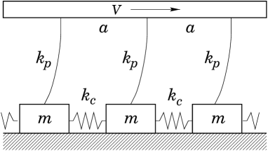
FIG. 1.: The Burridge-Knopoff model

Let us measure the displacement $X_{i}$ of the $i$-th block relative to the point of attachment of the $i$-th loader spring. In this case the total force $F_{i}$ acting on the $i$-th block is given by

$$F_{i}=k_{c}\left(X_{i+1}+X_{i-1}-2X_{i}\right)-k_{p}X_{i}-f_{i},$$ (1)

where $f_{i}$ is the force of friction. The dynamics of the system is completely determined by the equation of motion $m\ddot{X}_{i}=F_{i}$, provided that the friction law is specified. Note that the friction force $f_{i}$ is the only nonlinearity in the equation of motion. Clearly, the dynamics of the system will significantly depend on the particular choice of the friction law. Recently, a lot of results were presented on the dynamics of the Burridge-Knopoff model in the case of velocity-weakening friction law [9, 10, 12, 13, 14, 15, 16]. A characteristic feature of the Burridge-Knopoff model with this form of friction is its highly chaotic dynamics that occurs on all length scales down to the smallest length scale $a$ and therefore, the absence of the proper continuum limit [12].

In contrast to most previous studies, here we adopt the Coulomb friction law, which is applicable to clean dry surfaces (see, for example, [20]). Namely, we will characterize the friction force by the value of the static friction $f_{r}$ and the kinematic friction $f_{s}<f_{r}$, where $f_{r}$ and $f_{s}$ are positive constants. Thus, the block will remain at rest if $F_{i}<f_{r}$. When $F_{i}$ reaches $f_{r}$ the block starts to move (slips) and the friction force drops instantaneously from the value of $f_{r}$ to the value of $f_{s}$. When the block comes to rest (sticks), static friction turns on again. Also, we will supplement the friction force with the viscous friction term $f_{\mathrm{v}iscous}(v)=\alpha v$, where $v$ is the velocity of the block and $\alpha$ is a constant (Fig. 2).

FIG. 2.: Friction force as a function of the velocity

Note that this kind of friction law was considered already in the original paper of Burridge and Knopoff [11] and is observed in the friction experiments and their analogs [21, 22, 23, 24, 25]. Also note that this model was recently studied numerically in Ref. [17] (although for the parameters different from those considered in this paper).

We would like to emphasize that in contrast to velocity-weakening friction law, for which the kinematic friction force is a continuous function of the block velocity at $v=0$, in our friction law the force $f$ has a discontinuity at $v=0$, reflecting the fact that the coefficient of static friction is typically larger than that of kinematic friction. As a result of this difference, the accumulated stress accelerates the block at the onset of motion, releasing potential energy. As we will see below, this provides the sustaining force for the traveling waves studied in the following section. Also, as we will show below, this ensures the existence of the proper continuum limit as $a\rightarrow 0$.

Let us now formulate the equations of motion for the blocks in the case of the friction law introduced above. Recall that the displacements $X_{i}$ are measured relative to the loader plate, so they are defined in the reference frame moving relative to the surface with velocity $V$. Therefore, when the blocks are at rest, their equation of motion becomes

$$\dot{X}_{i}=-V.$$ (2)

When the block slides, its equation of motion changes to

$$m\ddot{X}_{i}=k_{c}(X_{i+1}+X_{i-1}-2X_{i})-k_{p}X_{i}-f_{s}-\alpha(\dot{X}_{i}+V).$$ (3)

The transition to sliding (slip) occurs when the force $F_{i}$ reaches the value of $f_{r}$:

$$k_{c}(X_{i+1}+X_{i-1}-2X_{i})-k_{p}X_{i}=f_{r}.$$ (4)

In other words, the equation of motion of a block changes from Eq. (2) to Eq. (3) when the condition in Eq. (4) is satisfied. Of course, the block comes back to rest when $\dot{X}_{i}=-V$ during sliding.

Let us introduce the following dimensionless quantities

$$x^{\prime}={x\over a}\sqrt{k_{p}\over k_{c}},~{}~{}~{}t^{\prime}=t\sqrt{k_{p}\over m},~{}~{}~{}u_{i}=-{k_{p}X_{i}+f_{s}\over f_{r}-f_{s}},$$ (5)

where $a$ is the distance between the attachment points of the loader springs (Fig. 1). The dimensionless displacement variable $u_{i}$ is chosen in such a way that the system is excitable only at $u_{i}>0$ [see Eq. (1), in order for slip to occur, the force $F_{i}$ must exceed the value $f_{s}$ of sliding friction], while the blocks will always slide for $u_{i}>1$ [see Eq. (4)].

If $k_{c}\gg k_{p}$, one can naturally go to the continuum limit by making a substitution $X_{i+1}+X_{i-1}-2X_{i}\rightarrow a^{2}{\partial^{2}X\over\partial x^{2}}$. This is a good approximation when the length scale of variation of $X_{i}$ is of order 1 in the new variables. Using the variables in Eq. (5), we rewrite Eqs. (2) and (3), respectively, as follows:

$$u_{t} = v,$$ (6)

$$u_{tt} = u_{xx}-u-2\gamma(u_{t}-v),$$ (7)

where we introduced dimensionless constants

$$\gamma={\alpha\over 2\sqrt{k_{p}m}},~{}~{}~{}v={V\sqrt{k_{p}m}\over{f_{r}-f_{s}}},$$ (8)

and dropped the primes for simplicity of notation. Note that in the continuum limit in addition to tracking the motion of individual blocks, one also has to follow the motion of the slip points. Similarly, one should keep track of the positions of the points at which the blocks come to rest. The latter are determined by the condition in Eq. (6) during sliding.

Determining the position of the slip points in the continuum limit turns out to be a rather complicated problem, since the position of the slip will still depend on the local dynamics of the blocks. In the discretized form, the slip condition [Eq. (4)] in the variables of Eq. (5) becomes

$${u_{i+1}+u_{i-1}-2u_{i}\over(\Delta x)^{2}}=u_{i}-1,$$ (9)

where $\Delta x=\sqrt{k_{p}/k_{c}}$. We will get back to this problem in the following section where we will show that in the continuum limit the dynamics of the slip becomes independent of $\Delta x$.

Equations (6) – (9) are the constitutive equations that will be studied in the rest of the paper. As can be seen from Eq. (5), we chose time and length scales so that the speed of sound in the system is equal to 1. The time scale is determined by the period of oscillations of an isolated block due to the loader spring. Note that in the continuum limit the characteristic speed of a block during sliding is much smaller than the speed of sound. This can be seen from Eq. (5) if one assumes $u_{t}\sim 1$, measures $X_{i}$ in the units of Eq. (5), and uses a natural assumption that $f_{r}-f_{s}\ll ak_{p}$. The behavior of the system is determined only by two parameters: the dimensionless dissipation parameter $\gamma$ which measures the effect of viscous friction, and the dimensionless rate of accumulation of stress $v$. In the following we will consider $v$ to be small, what expresses the fact that the time scale of accumulation of stress is much longer than that of the motion of an individual block during sliding.

Finally, let us discuss the applicability of the Burridge-Knopoff model in the context of real physical systems exhibiting stick-slip motion. In a real system one should replace a one-dimensional array of masses between the loader plate and the frictional surface by an elastic medium of certain thickness $h$. A straightforward extension of the Burridge-Knopoff model would therefore be a two-dimensional array of masses connected by springs whose one edge is rigidly attached to the loader plate and the other slides on the frictional surface. Naturally, the thickness of such a medium should greatly exceed the microscopic length scale $a$. The stick-slip motion in such a medium is due to surface waves [26]. The dispersion of these waves is given by $\omega^{2}=k^{2}+(\pi/2h)^{2}(1+2n)^{2}$, where $n$ is an integer and the transverse speed of sound was taken to be 1. The main difficulty here is that instead of a single displacement variable $u$ one has to deal with a large number of modes with different $n$. A simplification that is presented by the Burridge-Knopoff model consists of lumping up these modes into a single mode with an effective stiffness $k_{p}$ [Eq. (3)]. It is clear that the dominant modes will be those with small $n$, so we must have $k_{p}\sim(a/h)^{2}k_{c}\ll k_{c}$. Thus, in a physically relevant situation one should consider the continuum limit $\Delta x\rightarrow 0$ of the Burridge-Knopoff model. In short, this is merely a simplification of the mathematical handling of the elastic dynamics. A much more important assumption is that the friction response to the motion of the medium is instantaneous and has zero correlation length. It would be incorrect to think of the “size” of the block $a$ as an atomic distance. Rather, the value of the parameter $a$ should have a magnitude of the correlation (memory) length of the cooperative effects responsible for the surface friction (see, for example, [21] and references therein). Then the response of the system can be considered to be instantaneous if the characteristic velocity of the blocks is greater than $a/\tau_{\mathrm{s}tick}$, where $\tau_{\mathrm{s}tick}$ is the characteristic sticking time.

III traveling waves

Let us now demonstrate that Eqs. (6) – (9) admit solutions in the form of traveling shock waves with constant speed $c$ in the limit of vanishingly small $v$. But before we do that, let us see what kind of dynamics one would observe if there are no slip events and the initial distribution of $u$ is taken to be a sufficiently slowly varying distribution $u_{0}(x)$ (the latter ensures that no slip events will occur at short times). In this case the dynamics is trivial: we will have $u(x,t)=u_{0}(x)+vt$, as long as no slip events occur [see Eq. (6)]. From this one can see that the characteristic time scale of accumulation of stress is $v^{-1}\gg 1$, when $v$ is small. In other words, for $v\ll 1$ on the time scale of order 1 one will not see any motion with the distribution of $u$ fixed to $u_{0}(x)+C$, where $C$ is a constant. In particular, if one starts with the uniform initial conditions, one will have $u=u_{+}$, where $u_{+}$ is some constant less than 1. The other possible situation when the dynamics of the system becomes trivial is steady creep, when all the blocks move together with the loader plate, so we simply have $u=2\gamma v\simeq 0$ for $v\ll 1$ [see Eq. (7)].

Consider the system with $u=u_{+}$ and $v=0$. As was noted in the previous section, when $u_{+}<0$ slip events cannot occur, so if one slightly moves a particular block, it will quickly move to a new equilibrium position and no significant changes will occur. A different situation is realized for $0<u_{+}<1$ when the system becomes excitable. Then, if a single block is slightly moved, it will accelerate, releasing the potential energy accumulated in $u_{+}$. As a result of this acceleration, the force acting on the adjacent blocks will increase resulting in slipping of the adjacent block that was at rest. This avalanche-like process will go on, leading to the formation of the shock wave that releases the accumulated stress, so that $u$ changes to a new lower value of $u_{-}$. The situation here resembles a great deal combustion of safety fuse discussed in the Introduction. Thus, for $0<u_{+}<1$ a small perturbation of $u$ may lead to a significant change of the state of the system, switching it from $u=u_{+}$ to $u=u_{-}$. As in other excitable systems [1, 2, 3, 4, 5, 6], it is natural to expect that such a perturbation will transform at long times to a shock wave traveling with constant velocity $c$. Numerical simulations of Eqs. (6) – (9) with $v=0$ show that this indeed happens in our model.

Since all the “nonlinearity” in the problem is contained in the slip condition given by Eq. (9), our system is not unlike piecewise-linear model used to study propagation of nerve impulses [27]. For this reason the solution in the form of the traveling wave can be found exactly for $v=0$ in the continuum limit. For definiteness, we will consider the waves traveling from left to right, so that $c>0$. Because of the reflection symmetry, for each solution traveling with speed $c$ there is also a solution traveling with speed $-c$.

It is clear that the speed $c$ of the traveling wave should be determined by the motion of the slip point in front of the wave. Let the slip event occur for block $s$ at $t=t_{s}$. Then, for $i>s$ we have $u_{i}=u_{+}$, so the slip condition from Eq. (9) becomes

$$u_{s-1}(t_{s})=u_{+}-(1-u_{+})(\Delta x)^{2}.$$ (10)

Since at the onset of the slip $u_{s}=u_{+}$ and $du_{s}/dt=0$, at time $t$ we will have $u_{s}=u_{+}+{\cal O}\bigl{(}(t-t_{s})^{2}\bigr{)}$, with $u_{s}<u_{+}$, since right after the slip the block is accelerated by an excess force. This means that at some time $t_{s+1}$ the slip condition from Eq. (9) will be satisfied for the $(s+1)$-th block. According to Eq. (10), this will happen when $\Delta t=t_{s+1}-t_{s}={\cal O}(\Delta x)$. Therefore, on the time scale of order 1 this will correspond to the motion of the slip point with the speed $c=\Delta x/\Delta t={\cal O}(1)$.

To actually calculate the speed $c$ of the front, one needs to solve the system of coupled equations of motion for the blocks behind the $s$-th block. This problem in the limit $\Delta x\rightarrow 0$ is considered in Appendix A. The analysis of this problem shows that the speed $c$ of the wave is uniquely determined by the value of $u=u_{+}$ in front of the wave. Note that similar situation takes place in the models of combustion (see, for example, [18]) and in reaction-diffusion systems (see, for example, [1, 2, 3, 4, 5, 6]). The dependence $c(u_{+})$ found numerically is shown in Fig. 3.

FIG. 3.: The dependence $c(u_{+})$. Results of the numerical solution of Eqs. (A3) – (A7). Dashed line shows the result of approximation by Eq. (11).

We would like to emphasize that upon the decrease of $\Delta x$ the speed $c$ becomes independent of $\Delta x$, providing a well-defined continuum limit for slip propagation. These results are also supported by the direct numerical simulations of Eqs. (6) – (9).

According to Fig. (3), traveling wave solution exists for all $0<u_{+}<1$. The speed $c$ is always greater than 1, that is, the considered shock waves are supersonic. The latter is also observed in other models of stick-slip motion [15, 16]. Note, however, that the speed $c$ is the speed of propagation of the slip and is not related with the actual speed of individual blocks in the wave.

As can be seen from Fig. (3), the speed of the traveling wave diverges as $u_{+}$ approaches 1. One can get an analytical handle on the dependence $c(u_{+})$ by expanding it in the inverse powers of $c$ (see Appendix A). As a result, we get the following interpolation formula which implicitly determines $c$ as a function of $u_{+}$

$$u_{+}=\left(1+{2+c^{2}+4c^{4}\over 8c^{5}\sqrt{c^{2}-1}}\right)^{-1}.$$ (11)

This equation gives the dependence $c(u_{+})$ with a few per cent accuracy.

Let us introduce self-similar variable $z=x-ct$, where $c=c(u_{+})$ (Fig. 3). Since the problem possesses translational invariance, we can choose the position of the slip point to be at $z=0$. Similarly, the stick point $z=-w$, with $w>0$, will also travel with speed $c$ behind the wave. Behind the slip the blocks slide according to Eq. (7), so for the wave with speed $c$ we will have

$$(c^{2}-1)u_{zz}-2c\gamma u_{z}+u=0.$$ (12)

The slip condition gives the following initial conditions for this equation:

$$u(0)=u_{+},~{}~{}~{}u_{z}(0)=0.$$ (13)

The analysis of Eq. (12) (see Appendix B) shows that the structure of the solution changes qualitatively depending on whether the value of $u_{+}$ is smaller or larger than the critical value $u_{c}>0$, where the value of $u_{c}$ is implicitly determined by

$$\gamma={\sqrt{c^{2}(u_{c})-1}\over c(u_{c})}.$$ (14)

If we have $u_{+}<u_{c}$, the distribution of $u$ will asymptotically approach $u_{-}=0$ at $z=-\infty$ behind the wave [Fig. 4(a)].

FIG. 4.: Two types of traveling wave solutions: (a) case $u_{+}<u_{c}$; (b) case $u_{+}>u_{c}$.

In other words, the blocks behind the wave never come to rest. Therefore, upon passing of the wave the system should develop a steady creep for small but finite $v$. Note that this will always happen when $\gamma>1$ since in any case $u_{+}<1$, so for these values of $\gamma$ the propagation of multiple shock waves becomes impossible (see Sec. V).

A different situation takes place for $u_{+}>u_{c}$. Then the solution has the form shown in Fig. 4(b), and the width $w$ of the traveling wave becomes finite (see Appendix B)

$$w={\pi(c^{2}-1)\over\sqrt{c^{2}(1-\gamma^{2})-1}}.$$ (15)

Thus, in this case the wave propagates as a “self-healing” pulse (compare with [28]). Note that for $\gamma>0$ we have $c>c(u_{c})>1$, so the value of $w$ is bounded from below and the width of the wave is always greater or of order 1. This justifies the use of the continuum limit for $k_{c}\gg k_{p}$ and $\gamma\sim 1$. Furthermore, when $u_{+}$ becomes close to 1, the propagation speed $c$ and therefore the width of the wave grow, so in this case the continuum limit is justified even for $k_{c}\sim k_{p}$. On the other hand, the width $w$ goes to zero when $u_{+}$ becomes small when $\gamma\ll 1$ [see Eq. (15)], so for sufficiently small $u_{+}$ and $\gamma$ the continuum limit will become invalid for the description of traveling waves.

In the case $u_{+}>u_{c}$ the value of $u=u_{-}$ behind the wave will be (see Appendix B)

$$u_{-}=-u_{+}\exp\left(-{\pi\gamma c\over\sqrt{c^{2}(1-\gamma^{2})-1}}\right).$$ (16)

From this equation one can see that $u_{-}<0$, so right behind the wave the system is in the state in which no waves can be further excited. Also, note that when $u_{+}$ approaches the value of $u_{c}$, the value of $u_{-}$ rapidly approaches zero.

In the context of earthquakes a shock wave should be associated with an individual earthquake. The total displacement $A=u_{+}-u_{-}$ which occurs upon passing of a wave and which determines the magnitude of the earthquake will therefore be

$$A=u_{+}\left[1+\exp\left(-{\pi\gamma c\over\sqrt{c^{2}(1-\gamma^{2})-1}}\right)\right].$$ (17)

IV free boundary problem

So far we were studying traveling wave solutions in the limit $v=0$ and $u={\mathrm{c}onst}$ in front of the wave. These solutions are clearly the fast motions in the system since they occur on the time scales of order 1. On the other hand, although the accumulation of stress occurs slowly for $v\ll 1$, it can lead to significant changes in $u$ at long times of order $v^{-1}\gg 1$, so the latter can be associated with the slow motions in the system. Therefore, since the fast motions result in the large-scale changes in $u$, the slip-stick events can be considered as singular perturbations to the slow motions.

Similar situation is realized in other excitable media where the role of singular perturbation is played by the sharp fronts [1, 2, 3, 4, 5, 6]. A powerful tool in describing the dynamics of such systems is reduction to free boundary problem (see, for example, [18]). In this approach one obtains the relationship between the speed of the sharp front and slow variables. Using this idea, let us formulate the dynamics of our system as a free boundary problem.

Let us assume that the distribution of $u$ varies on the length scale much greater than 1. Then, introducing an adiabatic approximation, we can assume that the speed of the traveling wave is given by the dependence $c(u_{+})$ (Fig. 3) in which now, instead of $u_{+}$ one should use an instantaneous value of $u$ right in front of the wave. The latter will play the role of the slow variable. Thus, the motion of the shocks can be described by the variables $x_{i}(t)$ which give the positions of the $i$-th shock, and the variables $s_{i}=\pm 1$ which give the direction of their motion.

On large length scales the shock will contribute a discontinuity to the distribution of $u$ in the limit $v\rightarrow 0$. It can be included in Eq. (6) describing slow motions in the form of a $\delta$-function. Therefore, in the presence of the shocks Eq. (6) can be rewritten as

$$u_{t}=v-\sum_{i}c_{i}A(u)\delta(x-x_{i}+0s_{i}),$$ (18)

where $A$ is the amplitude of the shock from Eq. (17) evaluated at $u_{+}=u(x_{i}(t),t)$, $c_{i}$ is the absolute value of the speed of the $i$-th shock, and the last term in $\delta$-function represents the fact that the value of $u$ is evaluated right in front of the wave. Equation (18) simply says that at the moment $t$ the value of $u$ jumps from $u(x_{i}(t),t)$ at $x=x_{i}(t)$ to the new value $u_{-}(u(x_{i}(t),t))$ given by Eq. (16).

Having now defined the evolution of the slow variable $u$, we can write down the equation of motion of the shocks in terms of it

$$\dot{x}_{i}=s_{i}c_{i},$$ (19)

where $c_{i}$ is the function of $u_{+}=u\bigl{(}x_{i}(t),t\bigr{)}$ (Fig. 3).

Equations (18) and (19) are the basic equations of the free boundary problem describing the dynamics of the system for $v\ll 1$ and sufficiently slowly varying initial conditions, assuming that no creep occurs in the system during its evolution. These equations have to be supplemented with the way of dealing with creation and annihilation of shocks. From the physical considerations it is clear that a pair of shocks moving toward each other will annihilate. Similarly, when the value of $u$ reaches 1 [recall that our distributions of $u$ vary sufficiently slowly, so one can ignore the variation of $u$ in Eq. (9)], a slip event is initiated at the point where $u=1$, creating a pair of counter-propagating shocks. These features should be incorporated into the free boundary problem and will be discussed in the following section. Notice that according to Eq. (9) the distribution of $u$ for blocks at rest must be a continuously differentiable function in the continuum limit, so the speeds $c_{i}$ of the shocks given by Eq. (19) will also be continuously differentiable functions of time.

In writing Eq. (18) we assumed that we always have $u\bigl{(}x_{i}(t),t\bigr{)}>u_{c}$, so that the shock waves are always the waves of switching between the blocks with $u=u_{+}$ at rest in front of the wave to $u=u_{-}$ at rest behind the wave. In other words, we do not consider the possibility of the onset of creep behind the wave. The analysis of creep motion is beyond the scope of the present paper. The condition of the absence of creep should in fact be satisfied for a wide class of initial conditions. In particular, it is easy to see that a wave with $u_{+}>u_{c}$ will never be able to reach the points where $u<u_{c}$ if we have

$$|u_{x}|<{v\over c(u_{c})},$$ (20)

provided that the regions with $u<u_{c}$ are initially at rest. The condition in Eq. (20) simply means that the wave with speed $c$ will never catch up with the point at which $u=u_{c}$ when $u$ grows according to Eq. (6).

V spatiotemporal patterns

Let us now apply the procedure developed in the preceding section to spatiotemporal patterns forming in the system under consideration. As in any excitable system [1, 2, 3, 4, 5, 6], the basic pattern of this kind is a periodic array of shocks (wave train) traveling with constant velocity. From the results of the preceding section one can see that a periodic wave train should consist of sharp fronts in which the value of $u$ jumps from $u_{+}$ to $u_{-}$ followed by refractory regions where $u$ slowly recovers back to $u_{+}$, so the resulting pattern is saw-tooth (Fig. 5).

FIG. 5.: Periodic wave train.

In the refractory region $u$ obeys Eq. (6), which in the frame moving together with the wave with speed $c$ becomes $u_{z}=-v/c$, where $z=x-ct$ is the self-similar variable. Therefore, the solution for $u$ in the refractory region which properly matches with the back of one shock at $z=0$ and the front of another at $z=-L$, where $L$ is the period of the wave train, has the form $u=L^{-1}(z+L)u_{-}-L^{-1}zu_{+}$, where

$$L={cA\over v},$$ (21)

$c=c(u_{+})$ (Fig. 3), and $A$ is given by Eq. (17). Equation (21) should in fact be obvious from the purely geometric considerations. Thus, there exists a family of nonlinear periodic traveling wave solutions whose speed and period depend strongly on amplitude. Similarly, the period $T$ of this solution in time depends on the amplitude simply as $T=A/v$, so the frequency of the shocks at a particular point as the wave train passes is $\omega\sim A^{-1}$. The latter in fact represents a simple form of the Gutenberg-Richter scaling law with scaling exponent $b=1$ [29]. In other words, this exponent would be observed in the system under consideration if its dynamics were dominated by periodic wave trains. It is interesting to note that the value of $b$ actually observed from the earthquakes generally lies in the range $0.8<b<1.2$ [30].

The above arguments are justified as long as $u_{+}>u_{c}$, so that no creep develops behind the traveling front. Therefore, according to Eqs. (17), and (21), traveling wave trains exist only when $L>L_{\mathrm{m}in}$, where

$$L_{\mathrm{m}in}=v^{-1}c(u_{c})u_{c}.$$ (22)

Let us now consider another kind of spatiotemporal patterns that is typical of excitable systems — the source of counter-propagating waves [1, 2, 3, 4, 5, 6]. The existence of such a solution is associated with the fact that if there is an inhomogeneous distribution of $u$ at rest such that the maximum of $u$ is located at $x=x_{0}$, then at some point in time the value of $u(x_{0})$ may reach 1, so that the blocks will become unstable creating a pair of counter-propagating shocks (Fig. 6).

FIG. 6.: A source of counter-propagating waves.

After these shocks moved away from $x_{0}$, the distribution of $u$ can once again have a maximum at $x=x_{0}$, so after some time the value of $u$ will increase until it reaches 1 and the cycle repeats.

These solutions are indeed realized in our system. Close to $x=x_{0}$ we can approximate the distribution of $u$ as

$$u(x,t)\simeq 1-a(x-x_{0})^{2}+vt,$$ (23)

[see Eq. (6)], where we also assumed that the slip occurs at $t=0$. This time-dependent distribution of $u$ gives the values of $u$ in front of the shocks at $t>0$, after the slip occurred, thus determining the velocity of the shocks. The analysis of the free boundary problem in this case (Appendix C) then shows that right after the slip the positions of the shocks will be given by

$$x_{i}\simeq x_{0}\pm\sqrt{bt},~{}~{}~{}~{}~{}b={v+\sqrt{v^{2}+8a}\over 2a},$$ (24)

where the plus and the minus correspond to the shocks propagating to the right and to the left, respectively. Notice that Eq. (24) in general shows how to treat the singularity in the free boundary problem (Sec. IV) associated with the creation of a a pair of counter-propagating shocks.

The solution for $x_{i}(t)$ in Eq. (24) then allows to calculate the distribution $u^{\prime}$ after the shocks have passed

$$u^{\prime}(x,t)\simeq u_{-}(1)-a^{\prime}(x-x_{0})^{2}+vt,$$ (25)

where $a^{\prime}$ is given by (see Appendix C)

$$a^{\prime}=-a\kappa+{2av(1+\kappa)\over v+\sqrt{v^{2}+8a}},$$ (26)

$u_{-}(1)=-\exp(-\pi\gamma/\sqrt{1-\gamma^{2}})$ [see Eq. (16)], and

$$\kappa=\left(1+{\pi\gamma\over(1-\gamma^{2})^{3/2}}\right)\exp\left(-{\pi\gamma\over\sqrt{1-\gamma^{2}}}\right).$$ (27)

From Eq. (27) one can see that the value of $\kappa$ lies in the range $0<\kappa<1$. The plot of $a^{\prime}$ as a function of $a$ at a particular value of $\gamma$ is presented in Fig. 7.

FIG. 7.: Dependence $a^{\prime}(a)$ from Eq. (26) at $\gamma=0.3$.

From Eq. (26) one can see that there is a maximum of $u^{\prime}$ at $x=0$ ($a^{\prime}>0$) when the shocks have passed, if $a<a_{\mathrm{m}ax}$, where

$$a_{\mathrm{m}ax}={v^{2}(1+\kappa)\over 2\kappa^{2}}.$$ (28)

If this condition is satisfied, after time $T=v^{-1}\left(1+\exp\bigl{(}-\pi\gamma/\sqrt{1-\gamma^{2}})\bigr{)}\right)$ the distribution of $u$ will look exactly like the one in Eq. (23) which we started with, but with a different value of $a$. Therefore, Eq. (26) defines an iterative map for the value of $a$ corresponding to the solutions for $u$ at times $nT$, where $n$ is the number of iterations. Physically, a source with period $T$ will form at $x=0$ creating traveling waves propagating away from it. Note, however, that even though the period of the source is a constant that does not depend on the initial conditions, the solution represents an aperiodic process since after each cycle the value of $a$ changes. The latter is represented in Fig. 7. Observe that we always have $a^{\prime}<a$. From Fig. 7 one can also see that after many periods the value of $a$ will tend to zero. The analysis of Eq. (26) (see also Fig. 7) shows that zero is the only fixed point of the map $a\rightarrow a^{\prime}$ for any $\gamma$. For small enough values of $a$ Eq. (26) can be approximated as $a^{\prime}\simeq a[1-2a(1+\kappa)/v^{2}]$. It is then easy to show that after $n\gg 1$ iterations we will have $a_{n}\simeq v^{2}/[2n(1+\kappa)]$, where $a_{n}$ is the result of $n$ iterations of the map. Note that because of the fact that $a$ becomes smaller and smaller with each cycle, the distribution of $u$ becomes flatter and flatter [see Eq. (23)], what means that after a long time the regions in the neighborhood of the source will tend to synchronize. The characteristic size $R$ of a region in which the synchronization takes place can be estimated as $R\sim a_{n}^{-1/2}$, so we will have $R\sim t^{1/2}$. Also note that for the same reason if there are two sources with unequal values of $a<a_{\mathrm{m}ax}$ some distance $R$ apart, after time $t\sim R^{2}$ the one with the smaller value of $a$ will overwhelm the one with the larger value of $a$. It is then natural to expect that if the initial distribution of $u$ has all maxima with $a<a_{\mathrm{m}ax}$, the system will eventually synchronize into uniform oscillations in which all the blocks slide at once.

Different situation is realized when $a>a_{\mathrm{m}ax}$. In this case the distribution of $u$ forming after the shocks moved away from the origin will be a minimum rather than a maximum of $u$, so the next creation of a pair of shocks will not occur at $x=x_{0}$, but rather at different points in space. Therefore, it is natural to expect that for sufficiently random initial conditions one would see shocks created and annihilated at random points in space, creating a kind of spatiotemporal chaos.

VI conclusion

Let us now summarize the results of our analysis and discuss the relationship of our results with those obtained for other models of stick-slip motion. In the present paper we analytically investigated the Burridge-Knopoff slider-block model with Coulomb friction law, which is different from the one used in most previous studies [9, 10, 12, 13, 14, 15, 16]. This difference is expressed in the fact that our friction is a discontinuous function when the velocity of the block becomes zero. As a result, the system is capable of propagating ultrasonic traveling solitary waves in the limit of zero loader plate velocity for any value of accumulated stress above the excitability threshold $u=0$. The existence of such solutions is a characteristic feature of excitable systems [1, 2, 3, 4, 5, 6].

In the continuum limit the solution in the form of the traveling shock wave is independent of the short-scale behavior of the system, except for the precise form of the dependence of the wave’s velocity on the amount of the accumulated stress in front of the wave. The latter in fact only weakly depends on the dynamics of the model at short length scales if the value of $u$ is sufficiently close to the slipping threshold $u=1$. Note that one might want to calculate the dependence of the wave velocity on the amount of the accumulated stress $u_{+}$ by formally combining Eq. (12) at $z=0$ with the continuum version of Eq. (9) at $z=0$. This would give an incorrect result $c=1/\sqrt{1-u_{+}}$. This means that although the continuum approximation may be valid for finding the wave profile behind the slip point, one still needs to solve the discrete problem at the tip of the wave in order to find its velocity.

In the limit of vanishing loader plate velocity the only parameter in the model is the dimensionless coefficient of viscous friction $\gamma$. All our analysis was performed for arbitrary values of $\gamma$, so it is also applicable to the case $\gamma=0$, i.e., when the viscous friction is absent. This case, however, has one special feature. The thing is that for $\gamma=0$ we have $u_{c}=0$ [see Eq. (14)], so as $u$ approaches zero the speed of the wave approaches 1 and the width $w$ goes to zero [see Eq. (15)]. Therefore, for a fixed value of $\Delta x\ll 1$ the continuum limit will no longer be justified for the description of the waves when $u$ becomes sufficiently close to zero. Also, when $\gamma=0$ the amplitude $A=2u_{+}$ of these waves [see Eq. (17)] will be able to become arbitrarily small.

According to the results of our analysis, the solution in the form of the traveling shock wave, as well as a periodic wave train of a given period, is unique in the limit of vanishingly small loader plate velocity, and its speed is uniquely determined by the value of $u$ in the front of the wave. This is in contrast with the results of Langer and Tang [15] and Myers and Langer [16] for the models with velocity-weakening friction where they find a continuous family of such solutions and therefore a selection problem.

Note that the systems with velocity-weakening friction transform to the model considered by us in the limit of small $V_{f}$, where $V_{f}$ is the characteristic velocity of variation of the friction force. Indeed, if the characteristic speed of a block during the slip exceeds $V_{f}$, the friction force will drop very rapidly, acting in the same way as in our model. To obtain the criterion of smallness of $V_{f}$, we note that the effect of the velocity dependence of the friction is most pronounced in the slip region, where, according to Eq. (10), $u_{t}\sim\Delta x=\sqrt{k_{p}/k_{c}}$, where we assumed $c\sim 1$, so $u$ is not near the threshold value $u=1$. In the original variables $dX_{i}/dt\sim(f_{r}-f_{s})/\sqrt{k_{c}m}$, so the condition $V_{f}\ll dX_{i}/dt$ gives

$$V_{f}\ll{f_{r}-f_{s}\over\sqrt{k_{c}m}}.$$ (29)

This formula should in fact be obvious from the physical considerations. Similarly, one should recover our results for the creep-slip models considered in [7] if the characteristic velocity of variation of the friction force is small enough.

In contrast, if the condition opposite to the one in Eq. (29) holds, no traveling shock waves can be realized in the continuum limit. This can be seen from the following argument. In a traveling wave the profile of $u$ should be described by Eq. (12) in which, in the case of the velocity-weakening friction one should drop the term $-2c\gamma u_{z}$ and replace $u$ by $u-1$ close to the slip point. There we must have $u_{zz}<0$, so, according to the modified Eq. (12), we will have $c<1$ in the traveling wave. On the other hand, the propagation of subsonic waves in the system is impossible since from the dispersion relation $\omega^{2}=1+k^{2}$ for the waves in the absence of friction we get that their phase velocity $c=\omega/k=\sqrt{1+k^{-2}}>1$ for all $k$. On the other hand, numerical simulations show that in the discrete models with velocity-weakening friction traveling shock waves are indeed observed. However, for $\Delta x\ll 1$ these waves move with speeds very close to the speed of sound and their width is just a few lattice spacings (unless one is close to the threshold $u=1$, see also [15, 16]). One should therefore expect that in the continuum limit only discontinuous shocks traveling with the speed of sound are feasible, in contrast to the situation studied in the present paper. This is a crucial distinction of the Burridge-Knopoff model with velocity-weakening friction and the one with Coulomb friction law (Fig. 2) studied by us.

As was already discussed above, the propagation speed of the wave depends on the short-scale dynamics of individual blocks. Therefore, in order to be able to perform numerical simulations of the models under consideration in the continuum limit, one has to use very small discretization of time. This should make direct simulations of our model rather difficult. On the other hand, we showed that if the initial conditions vary sufficiently slowly, the dynamics of the system reduces to the motion of individual shock waves (see Sec. IV). Therefore, by reformulating the dynamics of the problem in terms of the free boundary problem one can dramatically increase the speed of the simulations, thus being able to observe the dynamics for much longer times. This should be important in the statistical analysis of our system, especially in the context of earthquakes (see also [12, 13, 14]).

Let us see how the results obtained from the studies of our model should translate to real stick-slip problems. Consider, for example, a Bristol board of thickness $h=2$ mm lying on the surface made of the same material under external pressure $p$ and pulled at the top [21]. The coefficients $\mu_{r}$ and $\mu_{s}$ of the static and the sliding friction for these surfaces were found to be $\mu_{r}=0.37$ and $\mu_{s}=0.31$, respectively [21]. The memory length which we should use for the distance $a$ between the blocks was found to be $a=1~{}\mu$m. A single block in the Burridge-Knopoff model should be associated with a piece of the board of dimensions $a\times a\times h$, so the mass $m$ of the block should be $m=2.4\times 10^{-12}$ kg, where we used the density $\rho=1.2~{}{\mathrm{g}/cm}^{3}$. From the speed of sound $c=a\sqrt{k_{c}/m}$ [Eq. (3)] we can calculate the values of $k_{c}$ and $k_{p}=k_{c}(\pi a/2h)^{2}$ (see the end of Sec. II). Using $c=4000$ m/s, we find $k_{c}=3.8\times 10^{7}$ N/m, and $k_{p}=2.3\times 10^{1}$ N/m. The friction force jump per single block is $f_{r}-f_{s}=pa^{2}(\mu_{r}-\mu_{s})$. One can see that the condition of Eq. (29) with $V_{f}=10^{-5}$ m/s (see [21]) is satisfied if $p=2\times 10^{6}{\mathrm{~{}}Pa}=20$ atm, what gives $f_{r}-f_{s}=1.2\times 10^{-7}$ N. For this value of $p$ the characteristic sliding velocity will be $\dot{X}\sim(f_{r}-f_{s})/\sqrt{k_{p}m}=1.6$ cm/s. The displacement $\Delta X$ in a single wave can also be estimated as $\Delta X=2(f_{r}-f_{s})/k_{p}=1\times 10^{-8}$ m. The latter quantity turns out to be quite small. Note that both $\Delta X$ and $\dot{X}$ increase as $p$ increases. Also, smaller pressures $p$ would be needed for smaller values of $h$. From [21] one can calculate $\alpha=6.7\times 10^{-6}$ kg/s for this value of $p$, leading to $\gamma=0.45$.

In the present paper we studied perfectly homogeneous system without any external noise. It is clear that in real systems some degree of noise should be present. It is interesting to know what effect the introduction of randomness will have on the behavior of the traveling waves. Here one can distinguish two different situations. If one adds some small randomness in the parameters of individual blocks, such as the friction coefficients, spring constants and so forth, one would expect the renormalization of the speed of the traveling waves. The other kind of noise would result in sudden transitions of the blocks at rest to sliding. This kind of noise can be readily incorporated into our free boundary problem by introducing generation of pairs of counter-propagating waves at random points in space. Here the open question is how the frequency of this generation should depend on the distance to the slipping threshold. It is also interesting how the presence of such a noise would affect the wave statistics.

A

Since the variation of $u_{i}$ leading to the slip event is of order $\Delta x^{2}$ and is small for small $\Delta x$, for the blocks near the slip point one can neglect both the variation of $u_{i}$ and the term $-2\gamma du_{i}/dt$ in Eq. (7), so in the limit $\Delta x\rightarrow 0$ the right-hand side of this equation simply becomes $u_{+}-1={\mathrm{c}onst}$. For convenience, let us introduce the new variables $\tau$ and $v_{i}$, such that

$$t=t_{s}+\tau\Delta x,~{}~{}~{}u_{i}=u_{+}-u_{+}(\Delta x)^{2}\left(v_{i}+{\tau^{2}\over 2}\right).$$ (A1)

Since at $\tau=0$ the $s$-th block just slipped, we must have [see Eq. (10)]

$$v_{s-1}(0)={1-u_{+}\over u_{+}},$$ (A2)

with the initial conditions

$$v_{s}(0)=0,~{}~{}~{}~{}v^{\prime}_{s}(0)=0,$$ (A3)

where the prime denotes the derivative with respect to $\tau$.

In the limit $\Delta x\rightarrow 0$ Eq. (7) can be written as

$${d^{2}v_{i}\over d\tau^{2}}=v_{i+1}+v_{i-1}-2v_{i}, ~{}~{}~{}~{}i<s,$$ (A4)

$${d^{2}v_{i}\over d\tau^{2}}=v_{i-1}-2v_{i}-{\tau^{2}\over 2}, ~{}~{}~{}~{}i=s.$$ (A5)

These equations essentially describe a linear array of unit masses connected by springs with spring constant 1, with the $s$-th mass attached to a rigid wall and acted upon by a time-dependent force $-\tau^{2}/2$.

If the wave moves with speed $c$, after time $\tau=1/c$, which corresponds to $\Delta t=\Delta x/c$ [see Eq. (A1)], it should move the distance $\Delta x$ to the right. This means that at time $t_{s+1}=t_{s}+\Delta t$ we must have $u_{i-1}(t_{s})=u_{i}(t_{s}+\Delta t)$, $u^{\prime}_{i-1}(t_{s})=u^{\prime}_{i}(t_{s}+\Delta t)$, or in terms of the new variables

$$v_{i-1}(0) = v_{i}(c^{-1})+{1\over 2c^{2}},$$ (A6)

$$v^{\prime}_{i-1}(0) = v^{\prime}_{i}(c^{-1})+{1\over c}.$$ (A7)

Note that these conditions introduce a feedback into Eqs. (A4) and (A5). Also, the solution of Eqs. (A4) should be matched with the continuum profile behind the tip, which satisfies Eq. (12). We should therefore have

$$v_{s-k}\cong{k^{2}\over 2(c^{2}-1)},~{}~{}~{}k\gg 1.$$ (A8)

Equations (A3) – (A7) can be solved numerically by an iterative procedure. Then, calculating the value of $v_{s}(c^{-1})$, using Eq. (A6) as a function of $c$, one can relate it to $u_{+}$ through Eq. (A2). The results of this numerical solution for $c>1$ are presented in Fig. (3). These results also show that close to $u_{+}=0$ we have

$$c\simeq 1+{1\over 2}u_{+}^{2}.$$ (A9)

The problem in Eqs. (A3) can be treated analytically by expanding its solution in the powers of $c^{-1}$. Indeed, if $c$ is large, for $\tau<c^{-1}\ll 1$ the right-hand sides in Eqs. (A4) and (A5) can be neglected, so the solution of Eqs. (A3) – (A7) for $k\geq 0$ in the leading order in $c^{-1}$ will be

$$v_{s-k}^{(0)}={k^{2}\over 2c^{2}}+{k\tau\over c}.$$ (A10)

Physically, this corresponds to the situation in which the springs between the blocks are absent.

To calculate the first order correction $v_{s}^{(1)}$, we use $v_{s-1}^{(0)}$ in Eq. (A5) to obtain

$$v_{s}^{(1)}={\tau^{2}\over 4c^{2}}+{\tau^{3}\over 6c}-{\tau^{4}\over 24}.$$ (A11)

This solution is then used to fix through Eqs. (A6) and (A7) the initial condition in Eq. (A4) with $i=s-1$ to the next order in $c^{-1}$. Using the solutions $v_{s}^{(0)}$, $v_{s-1}^{(0)}$, and $v_{s-2}^{(0)}$ in Eq. (A4), one can then calculate $v_{s-1}^{(1)}$:

$$v_{s-1}^{(1)}={3\over 8c^{4}}+{5\tau\over 6c^{3}}+{\tau^{2}\over 2c^{2}}.$$ (A12)

The knowledge of $v_{s-1}^{(1)}$ and $v_{s}^{(1)}$ then allows to calculate the next order correction $v_{s}^{(2)}$ by substituting them into Eq. (A5)

$$v_{s}^{(2)}={3\tau^{2}\over 16c^{4}}+{5\tau^{3}\over 36c^{3}}-{\tau^{5}\over 60c}+{\tau^{6}\over 360}.$$ (A13)

Substituting the obtained solution for $v_{s}$ into Eq. (A2) and using Eq. (A6) with $i=s-1$, we get

$${1\over 2c^{2}}+{3\over 8c^{4}}+{5\over 16c^{6}}={1-u_{+}\over u_{+}}.$$ (A14)

Note that this procedure can be continued to an arbitrary order in $c^{-1}$, although the calculation then becomes rather cumbersome. Let us only quote the result that the correction to the left-hand side of Eq. (A14) due to the next order terms will be $0.2719/c^{8}$.

Finally, combining Eq. (A14) with Eq. (A9), we arrive at the interpolation formula given by Eq. (11).

B

Here we solve Eq. (12) with the initial conditions given by Eq. (13) for arbitrary $\gamma$. Let us introduce the new variable $\xi=z/\sqrt{c^{2}-1}$ and a constant $\tilde{\gamma}={c\gamma/\sqrt{c^{2}-1}}$, where $c$ is a function of $u_{+}$ (Fig. 3). Then, Eq. (12) can be rewritten as

$$u_{\xi\xi}-2\tilde{\gamma}u_{\xi}+u=0,$$ (B1)

with the same initial conditions written in terms of $\xi$:

$$u(0)=u_{+},~{}~{}~{}~{}~{}u_{\xi}(0)=0.$$ (B2)

Two situations are possible here. If we have $\tilde{\gamma}>1$, both roots of the characteristic equation of Eq. (B1) are real, so the solution has the form

$$u=ae^{\xi(\tilde{\gamma}+\sqrt{\tilde{\gamma}^{2}-1})}+be^{\xi(\tilde{\gamma}-\sqrt{\tilde{\gamma}^{2}-1})}.$$ (B3)

Using the initial conditions from Eq. (B2), we obtain for the coefficients $a$ and $b$

$$a={u_{+}\over 2}\left(1-{\tilde{\gamma}\over\sqrt{\tilde{\gamma}^{2}-1}}\right),~{}~{}~{}~{}~{}b={u_{+}\over 2}\left(1+{\tilde{\gamma}\over\sqrt{\tilde{\gamma}^{2}-1}}\right).$$ (B4)

From the solution we see that behind the wave the distribution of $u$ asymptotically approaches zero. This means that we have $u_{-}=0$, but the system comes to rest only at $z=-\infty$, so the width $w$ of the wave is infinite. The form of the solution is shown in Fig. 4(a).

In contrast, when $\tilde{\gamma}<1$, the roots of the characteristic equation of Eq. (B1) become complex conjugate, so the solution has the form

$$u=ae^{\tilde{\gamma}\xi}\cos(\xi\sqrt{1-\tilde{\gamma}^{2}})+be^{\tilde{\gamma}\xi}\sin(\xi\sqrt{1-\tilde{\gamma}^{2}}).$$ (B5)

Substituting the initial conditions from Eq. (B2), we obtain

$$a=u_{+},~{}~{}~{}~{}~{}b=-{u_{+}\tilde{\gamma}\over\sqrt{1-\tilde{\gamma}^{2}}}.$$ (B6)

In constructing the full solution one should also take into account that the block will stick back when it comes to rest, what will happen when $u_{\xi}=0$ for vanishing $v$. According to Eqs. (B5) and (B6), this will occur at $z=z_{s}=-w$, where

$$w={\pi\over\sqrt{1-\tilde{\gamma}^{2}}}.$$ (B7)

Behind the stick point the value of $u$ will remain constant equal to $u_{-}$, with

$$u_{-}=-u_{+}\exp\left(-{\pi\tilde{\gamma}\over\sqrt{1-\tilde{\gamma}^{2}}}\right).$$ (B8)

Going back to $\gamma$, we can rewrite the equations above as Eqs. (15) and (16), respectively. The form of the solution in this case is shown in Fig. 4(b).

The solutions obtained above are the exact traveling wave solutions of Eqs. (6) – (9) in the case $v=0$. As can be seen from the construction, traveling wave solution is unique for any given value of $u_{+}$.

C

When a pair of counter-propagating shocks is created, their speed will be large, since in the neighborhood of $x_{0}$ the value of $u$ will be close to 1. This allows us to use Eq. (A14) and write

$$c_{i}\simeq{1\over\sqrt{2[1-u(x_{i},t)]}}$$ (C1)

for $x_{i}$ close to $x_{0}$. Note that Eq. (C1) expresses the fact that for $u$ close to 1 the coupling of the blocks through the longitudinal springs becomes inessential (see appendix A).

Without any loss of generality, we can put $x_{0}=0$. According to Eqs. (19) and (C1), we have approximately

$$\dot{x}_{i}=\pm{1\over\sqrt{2(ax_{i}^{2}-vt})}$$ (C2)

for not too large $|x_{i}|$ and $t$, with the initial condition $x_{i}(0)=0$. The solution $x_{i}(t)$ that satisfies this equation and the initial condition has the form $x_{i}=\pm\sqrt{bt}$, where the constant $b$ has to be determined. Substituting this expression for $x_{i}(t)$ into Eq. (C2), we obtain the following quadratic equation for $b$:

$$ab^{2}-vb-2=0.$$ (C3)

According to the definition of $b$, only the positive solution of this equation has physical meaning. Taking this into account, we obtain that the value of $b$ is given by Eq. (24).

From the solution of Eq. (C2) one can see that the shock reaches point $x$ at the moment $t_{i}(x)=x^{2}/b$. Right after the shocks have passed the new value of $u$ at the moment $t_{i}(x)$ is given by Eq. (16). Therefore, according to Eq. (6) the distribution $u^{\prime}$ at a point $x$ and time $t>t_{i}(x)$ behind the shock is given by

$$u^{\prime}(x,t)=u_{-}[u\bigl{(}x,t_{i}(x)\bigr{)}]+vt-vt_{i}(x),$$ (C4)

where $u$ is evaluated right before the shock reached $x$. Since $u$ in Eq. (C4) is close to 1, we can Taylor expand the dependence $u_{-}(u_{+})$ in this equation and keep only the first two terms. As a result, we obtain

$$u^{\prime}(x,t)\simeq u_{-}(1)+\kappa\left(ax^{2}-{vx^{2}\over b}\right)-{vx^{2}\over b}+vt,$$ (C5)

where $\kappa=-du_{-}/du_{+}$ evaluated at $u_{+}=1$. Using the explicit expression for $u_{-}$ together with Eq. (C1) in Eq. (16), one arrives at Eq. (27). Then, using the value of $b$ from Eq. (24), Eq. (C5) can be transformed to Eq. (25).

REFERENCES

- [1] M. Cross and P. C. Hohenberg, Rev. Mod. Phys. 65, 851 (1993).
- [2] V. A. Vasiliev, Y. M. Romanovskii, D. S. Chernavskii, and V. G. Yakhno, Autowave Processes in Kinetic Systems (VEB Deutscher Verlag der Wissenschaften, Berlin, 1987).
- [3] A. S. Mikhailov, Foundations of Synergetics (Springer-Verlag, Berlin, 1990).
- [4] Oscillations and Traveling Waves in Chemical Systems, edited by R. J. Field and M. Burger (Wiley Interscience, New York, 1985).
- [5] J. D. Murray, Mathematical Biology (Springer-Verlag, Berlin, 1989).
- [6] B. S. Kerner and V. V. Osipov, Autosolitons: a New Approach to Problems of Self-Organization and Turbulence (Kluwer, Dordrecht, 1994).
- [7] J. H. E. Cartwright, E. Hernández-García, and O. Piro, Phys. Rev. Lett. 79, 527 (1997).
- [8] M. A. Rubio and J. Galeano, Phys. Rev. E 50, 1000 (1994).
- [9] J. Schmittbuhl, J.-P. Vilotte, and S. Roux, Europhys. Lett. 21, 375 (1993).
- [10] P. Español, Phys. Rev. E 50, 227 (1994).
- [11] R. Burridge and L. Knopoff, Bull. Seismol. Soc. Am. 57, 341 (1967).
- [12] J. M. Carlson and J. S. Langer, Phys. Rev. A 40, 6470 (1989).
- [13] J. M. Carlson, J. S. Langer, B. E. Shaw, and C. Tang, Phys. Rev. A 44, 884 (1991).
- [14] J. M. Carlson, J. S. Langer, and B. E. Shaw, Rev. Mod. Phys. 66, 657 (1994).
- [15] J. S. Langer and C. Tang, Phys. Rev. Lett 67, 1043 (1991).
- [16] C. R. Myers and J. S. Langer, Phys. Rev. E 47, 3048 (1993).
- [17] H.-J. Xu and L. Knopoff, Phys. Rev. E 50, 3577 (1994).
- [18] P. C. Fife, Dynamics of Internal Layers and Diffusive Interfaces (Society for Industrial and Applied Mathematics, Philadelphia, 1988).
- [19] C. B. Muratov and V. V. Osipov, preprint patt-sol/9804001, LANL archive (submitted to Physica D).
- [20] F. P. Bowden and D. Tabor, Friction and Lubrication (Methuen, London, 1967).
- [21] F. Heslot et al., Phys. Rev. E 49, 4973 (1994).
- [22] Y. Brechet and Y. Estrin, Scripta Metall. 30, 1449 (1994).
- [23] B. D. Kilgore, M. L. Blanpied, and J. H. Dietrich, Geophys. Res. Lett. 20, 903 (1993).
- [24] M. A. Lebyodkin, Y. Brechet, Y. Estrin, and L. P. Kubin, Phys. Rev. Lett. 74, 4758 (1995).
- [25] S. Field, N. Venturi, and F. Nori, Phys. Rev. Lett. 74, 74 (1995).
- [26] L. D. Landau and E. M. Lifshits, Course of Theoretical Physics (Pergamon Press, London, 1959), Vol. 7.
- [27] J. Rinzel and J. B. Keller, Biophys. J. 13, 1313 (1973).
- [28] T. H. Heaton, Phys. Earth Planet Inter. 64, 1 (1990).
- [29] B. Gutenberg and C. F. Richter, Seismicity of the Earth and Associated Phenomena (Hafner Publishing Company, New York, 1965).
- [30] J. F. Evernden, Bull. Seismol. Soc. Am. 60, 393 (1970).