Induced Coherence and Stable Soliton Spiraling

Abstract

We develop a theory of soliton spiraling in a bulk nonlinear medium and reveal a new physical mechanism: periodic power exchange via induced coherence, which can lead to stable spiraling and the formation of dynamical two-soliton states. Our theory not only explains earlier observations, but provides a number of predictions which are also verified experimentally. Finally, we show theoretically and experimentally that soliton spiraling can be controled by the degree of mutual initial coherence.

Self-guided optical beams (or spatial solitons) have attracted substantial research interest in the last three decades [1]. Although interactions between two-dimensional (2D) solitons in Kerr and non-Kerr media have been studied extensively, only the recent discoveries of stable three-dimensional (3D) solitons in different nonlinear bulk media [2] initiated an experimental study of fully 3D interactions of solitary waves. Recently, experiments demonstrating non-planar interaction and spiraling of spatial solitons in a photorefractive medium have been reported [3]. However, in spite of earlier predictions of non-planar soliton interactions [4], the experimental results [3] have not been explained theoretically so far. Also, it has been shown [5] that coherently interacting solitons do not allow any stable spiraling, in sharp contrast with the experimental observations [3]. The fundamental question remains: Is soliton spiraling possible at all as a stable dynamical regime of soliton interaction?

In this Letter we develop, for the first time to our knowledge, a theory of soliton spiraling in a photorefractive-type nonlinear bulk medium. We derive an analytical model describing stable soliton spiraling and predict a number of new effects in soliton interactions, such as an induced coherence and control over 3D interactions, which we verify here experimentally, using experimental setup similar to that reported earlier [3]. Importantly, our analytical model and numerical simulations show that interacting-spiraling solitons conserve angular momentum. We believe that this result is a core foundation for future research on 3D soliton control, resembling the conservation of linear momentum in the interaction of more conventional (1+1)-dimensional solitons [6].

We consider incoherent beam interaction in an isotropic saturable nonlinear medium described by two coupled normalized nonlinear Schrödinger (NLS) equations

$$\begin{array}[]{l}{\displaystyle i\frac{\partial u}{\partial z}+\nabla_{\perp}^{2}u-\frac{u}{1+|u|^{2}+|w|^{2}}=0,}\\[9.0pt] {\displaystyle i\frac{\partial w}{\partial z}+\nabla_{\perp}^{2}w-\frac{w}{1+|u|^{2}+|w|^{2}}=0,}\end{array}$$ (1)

where $u$ and $w$ are the beam envelopes, $z$ is the propagation distance; $\nabla_{\perp}^{2}\equiv\partial^{2}/\partial x^{2}+\partial^{2}/\partial y^{2}$ accounts for the diffraction in the transverse ($x,y)$ plane. This system, in the 2D case (i.e., for $\nabla_{\perp}^{2}\equiv\partial^{2}/\partial x^{2}$), gives rise to incoherently-coupled soliton pairs [7] and to incoherent collisions [8] which have both been demonstrated with photorefractive screening solitons [9].

We look for solitary waves of Eqs. (1) in the form $u=U(r)\exp{(i\beta_{u}z)}$, $w=W(r)\exp{(i\beta_{w}z)}$, where the envelopes $U$ and $W$ satisfy the equations

$$\begin{array}[]{l}{\displaystyle\frac{d^{2}U}{dr^{2}}+\frac{1}{r}\frac{dU}{dr}-\beta_{u}U-\frac{U}{1+U^{2}+W^{2}}=0,}\\[9.0pt] {\displaystyle\frac{d^{2}W}{dr^{2}}+\frac{1}{r}\frac{dW}{dr}-\beta_{w}W-\frac{W}{1+U^{2}+W^{2}}=0.}\end{array}$$ (2)

Here $r\equiv\sqrt{x^{2}+y^{2}}$ is the radial coordinate, and $\beta_{u}$ and $\beta_{w}$ are nonlinearity-induced shifts of the propagation constants. System (2) has two families of soliton solutions: $U=G_{u}(\beta_{u},r)$, $W=0$ and $U=0$, $W=G_{w}(\beta_{w},r)$, which can be found numerically by solving the equation $G^{\prime\prime}_{\alpha}+G^{\prime}_{\alpha}/r-{\beta}_{\alpha}{G}_{\alpha}-{G}_{\alpha}/(1+G^{2}_{\alpha})=0$, where $\alpha=\{u,w\}$. These solutions can be characterised by the soliton powers $P(\beta_{\alpha})\equiv 2\pi\int_{0}^{\infty}G_{\alpha}^{2}(\beta_{\alpha},r)\;rdr$.

In addition to the one-component solitons, at $\beta_{u}=\beta_{v}\equiv\beta$ there exists a family of two-component (vector) solitons defined as: $U=G(\beta,r)\cos{\theta},\;W=G(\beta,r)\sin{\theta}$, where the variable $\theta$ characterises a power distribution between the components. Moving solitons of Eqs. (1) can be obtained by a well-known gauge transformation.

To study the soliton collisions analytically, we employ a Lagrangian formalism [10, 11]. Equations (1) can be obtained from the Lagrangian density: ${\cal{L}}=(i/2)(u^{*}u_{z}-uu_{z}^{*})-(|u_{x}|^{2}+|u_{y}|^{2})+(i/2)(w^{*}w_{z}-ww_{z}^{*})-(|w_{x}|^{2}+|w_{y}|^{2})-\ln(1+|u|^{2}+|w|^{2})$. Now we consider the interaction between two spatial solitons $(u_{1},w_{1})$ and $(u_{2},w_{2})$, taking $u=u_{1}+u_{2}$, $w=w_{1}+w_{2}$ and introducing the following free parameters $(j=1,2)$: the positions of soliton centers ($x_{j}$,$y_{j}$), and the common and relative phases of the soliton components $u_{j}$ and $v_{j}$, which we denote by $\phi_{j}$ and $\psi_{j}$, respectively. Following [11], we assume that the soliton parameters vary slowly in $z$, and integrate the Lagrangian density over $x$ and $y$. After this averaging procedure, we reduce the number of equations by using the conservation of the angular momentum, ${\cal M}=sV_{0}P/4$, where $s$ is the impact parameter (defined as the minimum distance between the trajectories of non-interacting solitons), and $V_{0}\equiv d{R}_{0}/dz$ is the initial value of the soliton relative velocity (see Ref. [5]).

The averaged Lagrangian can be presented as $L=L_{1}+L_{2}-U_{\rm int}$, where the first two terms are the individual contributions of the vector solitons, and the third term corresponds to an effective interaction potential given by

$${U_{\rm int}=M_{R}s^{2}V_{0}^{2}/(2R^{2})-U_{\rm incoh}(R)-U_{\rm coh}(R)\times}$$ (3)

$${\left[\cos{\theta_{-}}\cos{\phi_{-}}\cos{\left(\frac{\psi_{-}}{2}\right)}+\cos{\theta_{+}}\sin{\phi_{-}}\sin{\left(\frac{\psi_{-}}{2}\right)}\right]},$$ (4)

where $M_{R}\equiv P/2$, $\theta_{\pm}\equiv\theta_{2}\pm\theta_{1}$, $\phi_{\pm}\equiv\phi_{2}\pm\phi_{1}$, $\psi_{\pm}\equiv\psi_{2}\pm\psi_{1}$, and $R\equiv\sqrt{(x_{2}-x_{1})^{2}+(y_{2}-y_{1})^{2}}$ is the relative distance between the interacting solitons. The functions $U_{\rm incoh}$ and $U_{\rm coh}$ are expressed in terms of the soliton overlap integrals, $U_{\rm coh}=2\int\int_{-\infty}^{\infty}[G^{3}_{1}G_{2}/(1+G^{2}_{1})+G^{3}_{2}G_{1}/(1+G^{2}_{2})]dx\;dy$, $U_{\rm incoh}=\int\int_{-\infty}^{\infty}[G^{2}_{1}G^{2}_{2}/(1+G^{2}_{1})+G^{2}_{2}G^{2}_{1}/(1+G^{2}_{2})]dx\;dy$. The first term in Eq. (3) describes a centrifugal force (which is always repulsive), the second – incoherent attraction, and the third – coherent interaction. When $R$ is large enough, the soliton interaction is determined by the tail asymptotics $G(r)\sim\exp{[-\sqrt{(1+\beta)}r]}/\sqrt{r}$, that yields, $U_{\rm coh}(R)\sim\exp{[-\sqrt{(1+\beta)}R]}/\sqrt{R}$, $U_{\rm incoh}(R)\sim\exp{[-2\sqrt{(1+\beta)}R]}/R$ and $U_{\rm coh}\gg U_{\rm incoh}$. For smaller $R$, although $U_{\rm coh}>U_{\rm incoh}$, $U_{\rm incoh}$ is also important.

The average Lagrangian generates the following equations,

$${M_{R}\ddot{R}+\frac{\partial U_{\rm int}}{\partial R}=0,\;\;\;\;M_{\phi}\ddot{\phi}_{-}+\frac{\partial U_{\rm int}}{\partial\phi_{-}}=0,}$$ (5)

$${M_{\psi}\dot{\psi}_{-}-\cos{\theta_{+}}\sin{\theta_{-}}\frac{\partial U_{\rm int}}{\partial\theta_{+}}+\sin{\theta_{+}}\cos{\theta_{-}}\frac{\partial U_{\rm int}}{\partial\theta_{-}}=0,}$$ (6)

$${M_{\theta}\dot{\theta}_{\mp}\mp\frac{1}{2}\sin{\theta_{\pm}}\cos{\theta_{\pm}}\frac{\partial U_{\rm int}}{\partial\phi_{-}}\mp\sin{\theta_{\pm}}\cos{\theta_{\mp}}\frac{\partial U_{\rm int}}{\partial\psi_{-}}=0,}$$ (7)

where the dots stand for derivatives in $z$, and the effective masses are: $M_{\phi}=-{\partial P}/{\partial\beta}$, and $M_{\psi}=M_{\theta}=(\cos^{2}{\theta_{-}}-\cos^{2}{\theta_{+}})P$. First, we consider a reduced model assuming an additional symmetry, $\theta_{+}=\pi/2$. Then, the resulting system has stable stationary points. Solving this reduced system numerically we observe linear and even strong nonlinear oscillations near the stable minima. In general, the period of these oscillations in $R$ is different from the periods of $\theta_{-}$ and $\psi_{-}$. A stable stationary point corresponds to a smooth spiraling of the solitons.

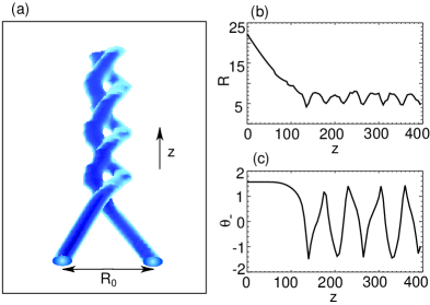
FIG. 1.: Stable soliton spiraling observed in direct modeling of Eqs. (1) for $\beta=-0.5$, $R_{0}=\sqrt{500}$, $s=10$, $V_{0}=0.2$, and $\theta_{-}=\theta_{+}=\pi/2$. (a) 3D view; (b) small oscillations of the relative distance between solitons; (c) large-amplitude oscillations for $\theta_{-}$ (quasi-periodic power exchange).

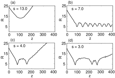
FIG. 2.: Examples of different dynamical regimes of the soliton interaction obtained by direct modeling of Eqs. (1) for $\beta=-0.5$, $V_{0}=0.2$, and $\theta_{-}=\theta_{+}=\pi/2$. The initial separation is defined as $R_{0}=\sqrt{400+s^{2}}$. (a) Weak soliton interaction (no spiraling); (b) stable spiraling; (c)(d) unstable spiraling (decay of spiraling configuration via resonances).

However, the analysis of the full dynamical system (5) brings a surprise: stable stationary points are absent. The main reason for this is the negativeness of the effective mass $M_{\phi}$ in Eqs. (5), which is a typical destabilisation mechanism for any coherent soliton interaction [5]. However, numeriacl simulations show that stable dynamical spiraling is still possible. To understand the physical mechanism of such a dynamical stabilisation, we analyse the effective interaction potential (3). Although $U_{\rm coh}>U_{\rm incoh}$ even for small $R$, large-scale periodic quarter-period out-of-phase oscillations in $\theta_{-}$ and $\psi_{-}$ can significantly suppress the effective value of the $U_{\rm coh}$ term, thus lowering its maximum value by a factor of $5$ or more. As a result, the incoherent attraction dominates and solitons become trapped in a spiraling configuration with oscillations near some $R_{\rm min}$ and large-scale quasi-periodic oscillations in both $\theta_{-}$ and $\psi_{-}$ (see Fig. 1).

Solving Eqs. (1) [and also (5)] numerically, we confirm the mechanism of the dynamical soliton spiraling. In summary, our theory and numerics show that

(i) Trapping of two beams in a stable spiraling is possible for a large range of parameters [examples are shown, e.g., in Fig. 1, for $s=10$, and Fig. 2(b), for $s=7$].

(ii) Initially mutually incoherent colliding solitons [i.e., $\theta_{\mp}(0)=\pi/2$] become partially coherent due to a periodic power exchange between their components. Moreover, stable spiraling is always accompanied by a large-scale periodic power exchange.

(iii) Initially introduced partial coherence between interacting solitons (seed mutual coherence) can result in repulsion of out-of-phase solitons and fusion of in-phase solitons, preventing spiraling.In this sense, modifying the initial mutual coherence can easily transform stable spiraling into repulsion (“escape”) or fusion.

(iv) For smaller $s$ and also for some values of $s$ where the spiralling and power-exchange frequencies become commensurable, the soliton spiraling is not possible [see Figs. 2(c,d)]. A series of ‘resonance windows’, similar to those discovered for 2D soliton interactions [12], are observed. For such values of $s$, oscillations in $R$ are stronger and $U_{\rm coh}$ can become dominant (even being effectively suppressed), thus leading to a decay of spiraling.

To verify our theory, we perform a series of experiments. The experiments are carried out using the photorefractive screening nonlinearity [3, 9]. In essence, the photorefractive nonlinearity is anisotropic [13], which makes it non-ideal to test our model. However, many experimental results suggest that for a large range of parameters, the anisotropy is fairly small: isolated 3D solitons are almost fully circular [14], and planar collisions between 3D coherent solitons are almost fully isotropic [15], except for a special case, e.g., when the collision plane is normal to the c-axis of the crystal and for a particular initial distance between the solitons [16]. In this respect, even though the photorefractive nonlinearity is not isotropic in 3D, one can still employ it to qualitatively study the predictions of our theory. We therefore extrapolate the known analytic results for 2D photorefractive screening solitons [9], which were all confirmed experimentally [17], to 3D which concurs with Eqs. (1).

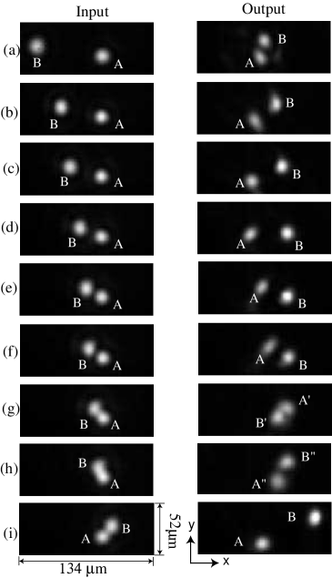
FIG. 3.: (a)-(i) Collision of two initially mutually incoherent solitons with different values of the impact parameter.

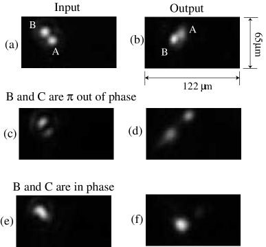
FIG. 4.: (a),(b) Stable soliton spiraling of initially incoherent beams. (c),(d) A “seed coherence” beam C, which is $\pi$ out of phase with B, prevents the spiraling; (e),(f) When the beam C is in phase with B, it causes all three beams to fuse.

The experimental setup is similar to that of Ref. [3]. Two soliton beams A and B of wavelength 488 nm, with power in the order of $\mu$W, and radii of 12$\mu$m FWHM are launched into an SBN crystal whose electro-optic coefficient is 278 pm/V and the length is 6.5 mm. The initial $y$ coordinate of B is 9 $\mu$m higher than that of A, and B is launched with its initial trajectory inclined (relative to that of A) by an angle of 0.01 radians in the $x$ direction and 0.0012 radians in the $y$ direction. The intensity ratio between the soliton peak and the background illumination, $|u|^{2}_{bg}=|w|^{2}_{bg}$, is about 5. A field of 4.2 kV/cm is applied against the the crystalline c-axis to generate the solitons. The impact parameter is adjusted by shifting the initial $x$ coordinate of B at the input, while all other initial conditions are kept unchanged. When the separation in the $x$ coordinate is larger than 31$\mu$m as shown in Fig. 3(a)-3(c), solitons A and B barely interact [compare with Fig. 2(a), which shows a passing of two solitons as if they do not interact at all]. As the impact parameter is reduced by shifting B closer to A, as shown in Fig. 3(d)-3(f), A and B’s trajectories are bent due to the attraction force between them, and the amount of bending (scattering) is dependent on the impact parameter. This mimics a classical particle scattering experiment. We distinguish A from B and measure the power exchange by monitoring the output within a time window much shorter than the response time of the SBN crystal (1 sec) after A or B is blocked. The measured power exchange is smaller than 1% in Fig. 3(a)-3(f).

When we further reduce the separation in the $x$ coordinate to 9$\mu$m [Fig. 3(g)], the two solitons rotate around each other [cf. Fig. 1 and Fig. 2(b)]. We find that 60% of A and 46% of B at the input go to A^′(at the output) and the rest goes to B^′. This power exchange is what we have called induced coherence. We also find that a small variation in B’s initial position or trajectory which does not change the rotation angle of beam trajectories by much, can cause the fraction of the exchanged power to vary considerably [compare with Fig. 1(c)]. In some spiraling cases, as low as a 5% level of power exchange has been measured at the output of the crystal. In a similar spiraling experiment, but with different initial trajectories, we find that the power exchange also depends on the intensity ratio. That is, the level of saturation of the nonlinearity. In that experiment, 17% power exchange is measured when solitons are generated with the intensity ratio of 12 and only 2% for the intensity ratio of 4.

We then reduce the $x$ separation further to 4 $\mu$m [Fig. 3(h)], and find that A and B interact strongly, but the spiraling seems to be unstable [compare to the numerical result shown in Fig. 2(c,d)]. Finally, when B is launched with its initial position beyond A [Fig. 3(i)], they simply escape from each other.

In order to study how the initial partial coherence affects the soliton interaction, we introduce at the input a “seed coherence” beam C which is coherent with B but overlaps entirely and copropagates with A. When C is added, the intensity of A is reduced to make the total intensity (A+C) equal to that of B. The relative phase between C and B is adjusted with a tilted piece of glass. Before C is launched, we make sure the initial conditions of A and B generate a spiraling pair [Figs. 4(a,b)]. When C is first adjusted to be out of phase with B [indicated by the dark notch between them at the input, Fig. 4(c)], B and A+C cannot spiral but just escape from each other, as shown in Fig. 4(d), although the power in C is only about 28% of A+C. When C is in phase with B, as shown in Fig. 4(e) (each intensity of A or C is 50% of B), A, B and C fuse into one beam [Fig. 4(f)]. These experimental results agree with our theory, emphasizing the fact that seed coherence can be used to control the interaction outcome: spiraling, “escape”, or fusion.

In conclusion, we have analysed fully 3D interaction and spiraling of spatial solitons in an isotropic saturable bulk medium. The analysis, numerical simulations, and a series of experiments have revealed the important physical mechanism of the stable spiraling: a periodic power exchange between the interacting beams via induced coherence. Our results and conclusions are expected to hold for other types of (even anisotropic and nonsaturable) nonlinearity that depends on the total beam power and supports stable self-trapped beams in a bulk.

A.V.B and Yu.S.K. acknowledge support from the Australian Research Council and the Australian Photonics Cooperative Research Centre. M-F.S. and M.S. were supported by the US Army Research Office.

REFERENCES

- [1] M. Segev and G. I. Stegeman, Physics Today (1998) August, and references therein.
- [2] M. Shih et al., Elect. Lett. 31, 826 (1995); W. E. Torruellas et al., Phys. Rev. Lett. 74, 5036 (1995); V. Tikhonenko et al., Phys. Rev. Lett. 76, 2698 (1996).
- [3] M. Shih, M. Segev, and G. Salamo, Phys. Rev. Lett. 78, 2551 (1997).
- [4] See, e.g., L. Poladian, A.W. Snyder, and D.J. Mitchell, Opt. Commun. 85, 59 (1991).
- [5] V. V. Steblina, Yu. S. Kivshar, and A. V. Buryak, Opt. Lett. 23, 156 (1998).
- [6] N. J. Zabusky and M. D. Kruskal, Phys. Rev. Lett. 15, 240 (1965)
- [7] D. N. Christodoulides et al., Appl. Phys. Lett. 68, 1763 (1996); Z. Chen et al., Opt. Lett. 21, 1436 (1996).
- [8] M. Shih et al., Appl. Phys. Lett. 69, 4151 (1996).
- [9] M. Segev et al, Phys. Rev. Lett. 73, 3211 (1994); D. N. Chirstodoulides and M. I. Carvalho, J. Opt. Soc. Am. B 12, 1628 (1995).
- [10] D. Anderson, Phys. Rev. A 27, 3135 (1983).
- [11] B. Malomed, Phys. Rev. A 43, 410 (1991).
- [12] D.K. Campbell et al, Physica D 19, 165 (1986); Yu.S. Kivshar et al., Phys. Rev. Lett. 67, 1177 (1991).
- [13] A.A. Zozulya et al., Phys. Rev. A 51, 1520 (1995); B. Crosignani et al., J. Opt. Soc. Am. B 14, 3078 (1997).
- [14] M. Shih et al., Opt. Lett. 21, 324 (1996).
- [15] H. Meng et al, Opt. Lett. 23, 897 (1998).
- [16] W. Krolikowski et al., Phys. Rev. Lett. 80, 3240 (1998).
- [17] K. Kos et al., Phys. Rev. E 53, R4330 (1996).